Differential Geometry of Curves: The Frenet Frame

[00:00:00]oddly satisfying about making  large swoops and fine squiggles.

[00:00:09]People have been fascinated  by curves since antiquity, as evidenced by neolithic cave  paintings and carved stones.

[00:00:19]Curves appear all around us in nature: in the  arcs of planets and stars sweeping across the sky, in twisting vines, meandering  streams, and in snail and seashells.

[00:00:34]Modern day examples include roller coasters and  water slides, railroads and freeway interchanges, and mechanical springs of all kinds. Today,  we'll break down what a curve is mathematically: how they are defined, and how to measure how  curvy they are in both two, and three dimensions.

[00:00:56]We'll learn how if you're given a curve, you  can define a kind of privileged reference frame, or basis, at every point on that curve that has  applications in differential geometry, aerospace, and more. We'll also see that nice enough curves  -- in a way we'll make precise later -- turn out to be determined by just two functions, despite  living in three dimensions. Let's get started!

[00:01:23]The simplest curve that actually curves is the  circle, so let's start there. Here's a circle.

[00:01:32]It's the set of all points within a plane a  fixed distance from a point called the center.

[00:01:37]Defined in this way, the circle has no start or  end -- it just sits there in all its roundness.

[00:01:44]But often when mathematicians say curve,  they mean not just the completed drawing, but a function that traces out the curve  over time. This is called a parameterization.

[00:01:57]The individual functions of the  parameterization are called component functions. Despite the different  looking expression for the curve from the earlier equation, the  resulting image is the same.

[00:02:12]Throughout this video we'll restrict our  attention to smooth curves, meaning we can safely take derivatives as many times as we like.  To take the derivative of a parametrized curve, simply take the ordinary derivative  of each component function. The first derivative at some point tracing the curve can  be visualized as a tangent vector at that point whose length or magnitude is the  speed of the point at that time.

[00:02:40]Think of this first derivative as the velocity.

[00:02:45]Shown here is a point going around the circle at  varying speed, like a caterpillar inching along.

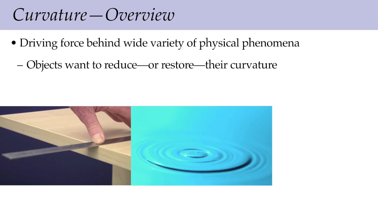
[00:02:52]However, for simplicity, we'll usually work  with curves parameterized to unit speed, meaning the magnitude of the derivative is  constantly one. This focus on unit speed curves doesn't really reduce the scope of curves  we're investigating, because theory tells us that the image of any smooth curve can be obtained by a  unit speed curve instead. Now take a look at these circles. What makes them different? Intuitively,  it feels like a small circle has greater curvature than a large circle; after all, as the radius  of the circular road increases, it feels closer and closer to driving on a straight road with  no curvature. How might we define curvature?

[00:03:32]One way you might be thinking is to define  curvature to be the reciprocal of the road's radius. That way a large circle has small  curvature, whereas a small, tight circle has high curvature. Another strategy is to ask at what  rate the angle of the car rotates per unit time.

[00:03:54]Yet another idea is to appeal to physical  intuition and argue for defining curvature as the magnitude of the acceleration  as you make the turn at constant speed.

[00:04:07]Believe it or not, these approaches actually  turn out to be equivalent! We will stick to the last definition in this video, as it  most easily generalizes to other curves.

[00:04:19]Let's try an example. Consider  this parametric circle formula.

[00:04:25]Here's the derivative, and its magnitude is v.  So this parametrization has constant speed v.

[00:04:33]Let's compute the curvature using the magnitude  of acceleration definition. The acceleration is the second derivative shown. Notice the  acceleration is perpendicular to the velocity, which should match your intuition. Taking the  magnitude, we get v squared over R. Requiring our circle to have a unit speed, v equals one,  means its curvature is actually one over R.

[00:04:57]Implicit in this calculation is the reason  it's standard to only define the curvature for unit speed parameterizations. If we use a  curve with a different speed, its magnitude of acceleration will also be different, changing  the value of the curvature. But we really want the curvature to only depend on the image of the  curve. We call the curvature kappa for short.

[00:05:21]By defining the curvature to be the  magnitude of the second derivative we can work out the curvature of any smooth unit  speed curve. As in the special case of a circle, the curvature of a smooth curve has a number  of ultimately equivalent interpretations: it's the size of the second derivative,  the rate of change of the turning angle, the reciprocal of the radius of the best  fitting circle to the curve at that point, and the local deviation of the  curve from being a straight line.

[00:05:52]Now, if gamma is a parameterized straight  line, which technically counts as a curve, its second derivative is identically zero, so  its curvature is zero as well, as we would hope!

[00:06:07]Here's one more example of a unit speed curve:  it's a spiral, and the constant b determines how tightly it winds. If you'd like to take on the  challenge of calculating its curvature yourself, pause the video here and take a few minutes, and don't forget to confirm it's really  unit speed. All right here we go.

[00:06:33]The first derivative involves using the  product, and chain rule. Writing it down, it looks like an awful mess at first, but a lot  of it fortunately simplifies to an expression that is easily verified to have magnitude 1. The  second derivative is much easier than the first, resulting in an expression whose magnitude is  b over t. This is the curvature of the spiral.

[00:06:55]With the definition of curvature for unit speed  curve in hand, we're ready to tackle 3d curves as well. Such a curve is defined by a parametric  equation with three coordinate functions.

[00:07:08]We call it a space curve to distinguish it  from the plane curves we looked at previously.

[00:07:15]As mentioned earlier, taking the derivative  yields the tangent vector to the curve.

[00:07:20]In the case of a unit speed curve, this  tangent vector has length 1 by definition.

[00:07:26]We'll call this unit tangent capital T.

[00:07:31]The fact that t is unit length can be nicely  expressed with the dot product T dot T equals 1.

[00:07:40]Now for some calculus. We can take the  derivative of both sides of the last equation using the fact that the dot product  obeys the usual derivative product rule.

[00:07:52]Further, since the dot product is symmetric,  we can rearrange and combine the two terms.

[00:07:59]When the dot product of two vectors is zero,  they're perpendicular, so we've just shown that T prime, the second derivative of the curve,  is perpendicular to T. While T has unit length, T prime generally doesn't. But, as long as  T prime is non-zero, we can normalize it to get a unit length vector perpendicular  to T. We make this idea into a definition: N equals T prime divided by the magnitude of T  prime. The factor of magnitude of T prime should look familiar: it's the curvature kappa of our  curve. N is called the unit normal. Currently, we have a pair of perpendicular unit vectors  T and N at every point of our space curve.

[00:08:50]Since we're in three dimensions, we need a third  vector to make a basis. Taking their cross product T cross N results in another unit vector  that's perpendicular to both. This third vector is denoted B and called the binormal. By  construction, the set {T, N, B} is an orthonormal basis for the space of all possible vectors  attached to any given point along the curve. But it's not just any orthonormal basis, it's derived  from the curve in a geometrically meaningful way.

[00:09:27]{T, N, B} is called the Frenet Frame of the curve.  Keep in mind that the unit normal N, and hence the whole Frenet Frame, is only well defined if the  curvature is non-zero. As a point traces out a parameterized curve, It's attached Frenet Frame  also dynamically moves. Key geometric information is revealed when the motion of the Frenet Frame  is expressed in terms of the Frenet Frame itself.

[00:09:59]How do we investigate the motion of  the Frenet Frame in terms of itself?

[00:10:03]Well, as usual, motion is encoded by derivatives, so the plan is to compute T prime, N prime,  and B prime, and express them in the bases T, N, and B. Recall that N is the normalized  version of T prime. Explicitly, T prime equals κN. This expresses T prime in the Frenet Frame  using N, while T and B make no contribution yet.

[00:10:35]Now for N prime. Since N is unit length, N  dot N equals 1. By the exact same argument that showed T prime is perpendicular to T, it's  also true that N prime is perpendicular to N.

[00:10:52]This means N prime is a combination of T and B  -- the only other directions available. Formally, T prime equals c_1 times T plus c_2  times B for some real numbers c_1 and c_2 since c_1 is the coefficient of N prime  in the direction of the unit vector T, we can find it by computing N prime dot T.  As a first step, we have N dot N equals zero.

[00:11:23]Taking the derivative of both sides gives us  N prime dot T plus N dot T prime equals zero.

[00:11:30]Now remember T prime equals κN.  Substitute this into the last equation.

[00:11:37]Since N has unit length, we get N prime dot T plus  κ equals zero. So it turns out c_1 is equal to minus κ. The coefficient c_2 is a new quantity  that we have no good way of rewriting in terms of known ones. Traditionally, the symbol used for  this coefficient is τ and it's called the torsion.

[00:12:04]we'll see that torsion encodes the twisting  of the curve along its direction of motion.

[00:12:10]We now have the equation N prime equals minus  κT plus τB, which takes care of writing N prime in the Frenet Frame. One more to go! Finally, we  take on B prime. By definition B equals T cross N, and like the dot product, the cross product  also obeys the usual derivative product rule.

[00:12:39]Substitute in our previously found expressions  for T prime and N prime. Remember that any vector crossed with itself gives zero, and  T is unit length. Lastly, apply the right hand rule to work out T cross B. Putting all  this together we find B prime equals minus τN.

[00:13:07]in summary T prime equals κN, N prime equals minus  κT + τB, and B prime equals minus τN. We've done it! These are the famous Frenet-Serret formulas:  differential equations discovered independently by Jean Frédéric Frenet in 1847 and Joseph  Alfred Serret in 1851. These formulas are a cornerstone of the differential geometry of  space curves. In fact, they can be used to completely characterize space curves with non-zero  acceleration everywhere (to make sure N and B are defined). But before we get to that, what  are these formulas saying? And what is this τ?

[00:14:00]Toward answering this, consider the plane  spanned by T and N at some point known as the osculating plane. Our earlier interpretations of  the curvature for plane curves still apply within this plane. In particular, the first Frenet-Serret  formula T prime equals κN says the rate of change of the tangent vector is in the direction of the  normal with magnitude equal to the curvature.

[00:14:28]Intuitively, the curvature encodes the rate of  steering left and right from the perspective of the moving point within the osculating plane.  But now we also have this quantity τ, the torsion.

[00:14:44]We can think of τ as analogous to κ, but  acting on the entire osculating plane instead of just the tangent vector. Let's  look at the third Frenet-Serret formula B prime equals minus τN. It says the binormal moves  toward or away from the normal with magnitude τ.

[00:15:05]Equivalently, this means the osculating plane  rotates about the axis of the tangent T.

[00:15:12]If τ were zero, there would be no rotation of  the osculating plane, and so the curve would remain in that plane -- that is, it would be a  planar curve, like the ones we saw initially.

[00:15:25]Here's another way of thinking about these things.  Suppose you're the pilot of a plane flying around in 3d space. Using the control yoke, you can steer  the plane horizontally left and right (called yaw, in flight jargon), pull the nose of the plane  up or down (called pitch), or do a barrel roll (called roll, appropriately enough). Each of these  movements is a rotation around a certain axis.

[00:15:54]How are these related to curvature and torsion?  Well, we can think of yaw as representing curvature and roll as representing torsion.  For example, here the plane is just yawing to the left, now it begins to roll clockwise......right about here, while still yawing.

[00:16:18]The result is the plane gaining height above the ground, just  like pitching up.

[00:16:23]to work its way into pop culture in the 2016 film  Hidden Figures, about some heroic women working to calculate rocket trajectories -- which are quite  literally space curves -- for nasa in the 1960s.

[00:16:39]Ruth, uh... get me the... Do you think you can find me the Frenet  Frame for this data using the Gram-Schmidt......orthogonalization algorithm? Yes sir.  I prefer it over euclidean coordinates.

[00:16:56]Given a choice of two continuous functions  κ, (which must be positive), and τ, (which is allowed to be zero or negative), there is a  space curve having that curvature and torsion.

[00:17:09]Moreover, this curve is essentially unique in  that if another curve also has that curvature and torsion, these curves will be directly isometric.  This means a translation and rotation of space will take one curve to perfectly overlap the  other. The proof of this theorem is beyond the scope of our video, but roughly it starts  with the Frenet Serret formulas, and applies the existence and uniqueness theorem for the  solutions to ordinary differential equations.

[00:17:42]The upshot of it is we can generate an essentially  unique curve given the starting data of a pair of functions κ and τ and further we can tell if two  curves are essentially the same by computing their curvature and torsion. This result is deservingly  called the Fundamental Theorem of Space Curves.