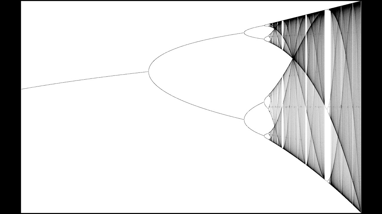
Feigenbaum Constants, Lyapunov Exponent, and Renormalization

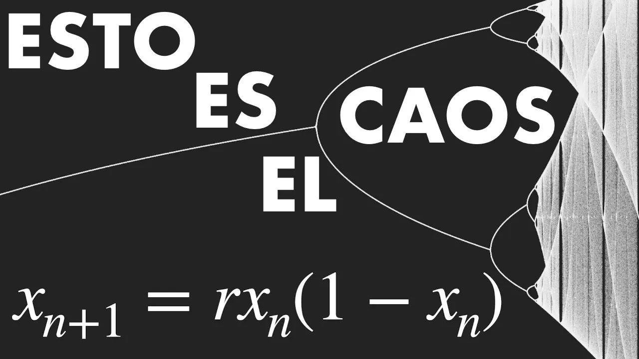
[00:00:00]our analysis so as you can see if I increase this value the points get away from each other right and then you can see that at the next bifurcation point which happens around 3.4 something it's the same story okay if you remember in the previous bation this was minus one and the second order function's derivative was one this time FS2 is min-1 and F 4 is one and there is another bifurcation and if you can see it this function looks off a lot like itself do you see it some uh fractal stuff coming your way in really fast so how how does it look like itself imagine this whole function and then just take you see this goes up then there is this uh Castle here right and then then if you look here in Reverse it goes up then there is a castle here do you see that yeah so it's as if this function is itself but shortened rotate it put it down right self similarity so this looks an like what like um the TR PR series step function what step for your St function trans so taking the pite um it's almost like we have taken just the pite in terms of re some punish ah I see very good very good uh what was this one okay I will come to that one soon well as I mentioned we do understand why those periodic Windows appear uh they appear for example if you plot F3 versus X the period 3 appears when the function just barely touches this line okay and you might think that finding this is very easy actually there's a story here one can show analytically that the value r at the tangent bation is this so when R is 1 + < TK 8 you have that period 3 window appearing this beautiful result is often mentioned in textbooks and article but always without proof given the resemblance to this result that is for another thing I'd always assume it should be comparably easy to derive and once assigned it as a routine homework problem oops turns out to be a beer bear no I I don't I okay there's there's bear with me there's the beer there's the beer I don't know how to read them but in any case this is also is a part where you have this intermittency meaning that things go rather in an ordinary way except for some burst of activity in between so that's another way of going towards chaos it's called intermittency route to chaos but we will focus on uh we will focus on period doubling root to CS what do we mean by that let me just find the relevant place here okay so it turns out that there is some mathematics some geometry hidden here let me show you how you have a bifurcation here right the next bifurcation is here the next bation is here the next one is here and they get closer and closer right so fim bound realized that if you take these distances like between the first bifurcation and the second bifurcation let's call it Delta n and let's say the second one and the third one is Delta n + 1 and if you take Delta n over Delta n + 1 and take limit n goes to Infinity meaning that it bifurcates smaller and smaller smaller and smaller smaller and smaller it converts to a universal number okay magic let me remind you we started with a simple function Lambda x 1 - x then we saw bifurcations we were surprised now we are seeing that there is some geometry hidden in that bations and this number has nothing to do with e Pi or any mathematical constant that we know it's another mathematical constant it's a mathematical constant of chaos okay why it's a mathematical constant because as you will see in your homework uh your homework is to look at this map okay and change mu so you will see the same kind of bifurcations while you change me of course the values of those bifurcations will be at different points but you will if you do it correctly you will see that as you get closer and closer to bifurcation Point uh the chaos Point uh the points where that bifurcation happens if you take the ratios it converts to the same exact value so a different map and it turns out that as long as you have one hump on your function and as long as that hump is quadratic you will get the same values okay that's not where it ends though there is another Universal constant and let's define it like this this is the maximum point of the plot okay the maximum point of the plot over here x maximum if we look at the distance from this point to the closest bifurcation Point okay do you see that it gets smaller and smaller but it also alternates and gets smaller and smaller now if you do that one DN + 1 / DN as n goes to Infinity you will get another Universal constant Etc now we will derive this constants and we will try to understand what it is all about okay um okay so let me first we we'll come to that point let me first tell you where that there is an encyclopedia in the internet the online encyclopedia of integer sequences okay a lot of fun so you can find pi here or other stuff like that but this is a sequence 3.56 99456 7 one8 Etc what is this this is the point where all those bifurcations uh approach to you know period double double again double again double again double again until you hit exactly this point where you exactly start the cows and we will be able to exactly pinpoint this point of chaos with some methods okay but let's say we did it let's say we know the number infinitely many digits of it let's actually plot our function as it goes closer to it and I'm going to PL uh let me gather my thoughts together uh what I have here this one this one this one let me just plot it like this okay this is already ruining the surprise so give me a moment to think okay okay I thought about it and I'm plotting it again I will explain everything will be all right just wait for this plot okay here it is now what is nice about this plot you see with this plot we had to zoom in and every time we zoomed in we have lost the quality of the plot right you remember that now what we are doing instead is we know where it hits the cows right so we are approaching that point logarithmically meaning that the X point is minus of the logarithm of R critical minus r who can explain me what is going on here anyone so what is zero here r c r rc- r = e to the power of Z right very good 2 means RC minus r is equal to E to Theus 2 this one means RC minus r so we are really really close but we as we get closer we approach slower so the fact that these distances now seem to be equal is just telling us that our approach is geometric okay as you go closer and closer you have to travel the same amount of distance in the exponential to get to the next bifurcation uh now I I should be able to zoom look if I zoom here you get the same story Zoom here you get the same story Zoom here you get the same story and this distance over here from here to here what is this distance can you tell me approximately 1.6 or something like that right let's do MP exponential 1 1.6 do you see it's very close to the universal constant 4.

[00:12:48]669 do you understand it do you understand why this is the case no right okay let me explain this is RC uh this is the way that we see this plot right so let's say this is rx uh no let's say this is um what was it 9.8 right this is 9.8 and this point is what 8.3 okay so it is telling you that the ratio of this one to this one is so one of them is R let's let me just call this one R1 R2 R3 R1 is equal to rc minus E to Theus 8.3 R2 is equal to r c minus E to the- 9.8 R3 is equal to rc minus E to- 9.8 uh minus 1.5 which is what 11.3 did you follow this yes so what are we looking for we are looking for R3 minus R2 over uh I have to be careful is this what we are looking for no we are looking for R2 - R1 R3 - R2 I think this is better please help me out no one is going to help me out I think the above one should be reverse should be e the 9 look hear me out hear me out do you agree that this is much smaller than the other one this is much smaller than the other one so if you divide them it's approximately e to the 1.5 that's what's going on so we don't need to approximate in both cases we can exactly exactly you can factor out 1 minus e to the power of something and you are going to exactly get e to the 1.5 are you happy yes yes good so this distance tells us something so that distance tells us the first fum bound constant actually people call it fan value okay I'm glad that you smiled at least once during this course uh so we we got the idea about first fan value what is uh what is the intuition for the second Fen value so if you remember it was the distance from the maximum of the plot so let's do the following the maximum of our plot is XM equal to 0.5 that's where it's maximized so I'm going to plot let me plot uh not the logarithm just absolute value first just absolute value of the AIS okay do you see what I did whenever it's below 0.5 it's flipped up okay now do you see this point H now there self simility here exactly now there is a self similarity you can see this plot is basically this plot basically this plot basically that plot but it's getting smaller and smaller shrinking so the point where we are going to concentrate is these points do you see this point goes down then goes down by similar amount right so if I plot it in log again also that axis it's going to be cool okay let's do that in log and I have never seen anyone plot it this way so you are you don't feel it right now but you are really lucky there you go now it's now you have one plot which is in log log and it has two both Fen values in it the first F value we already discussed corresponds to the distance between this point and this point and that's around 1.5 and that corresponds to 4.69 whatever the second F value is okay the distance in the vertical Direction so this distance this one with respect to that one because remember it was going down logarithmically and I plot it in logarithm so it now goes down linearly sorry it was going down exponentially I took the logarithm so it now goes down linearly what how about these numbers what is this number 7.5 something let's just focus 7.45 remember that now I go to the next one okay sorry so 7.45 what is this one 7.45 what is this one 8.35 something like that right 0.9 okay okay uh it's very close to 2.5 right but we will get so good at it that we will eventually get all the digits do you see very nicely let's let's get super good at it let me show you the final code uh for final code to work I actually have to go to higher precisions in decimals like to 32 precisions what this code is doing is finding the precise position of the bifurcations and finding the distances and if you run this code in 38 seconds it finds the relevant f f Mound constants you can see it goes closer and closer to those values and what we are using here have you heard of binary search yes yes one thing that we are using is binary search but I have to explain you so many things to for it to make sense um okay okay let me think so here is how it starts R1 is three do you remember three was the first place where it bifurcated where do we expect the next bifurcation to happen we expect it to happen um ah we don't need to expect it we actually find it by this function find bifurcation point and we are just giving it where where we expect it to happen we expect it to happen between 3.4 and 3.5 okay and it finds that value exactly now how does it do that if we go to find bifurcation Point function this is how it works and find bifurcation Point actually depends on derivative at fixed point and the derivative at fixed Point depends on finding fixed point and this is find fix Point function are you still with me no Inception come on you don't need to do that face okay let me give you this is too hard right okay let's go back to some Concepts I will talk about something very important this is leonov exponent so let's go back to our book talk about leonov exponents where is it oh I have also renormalization so much fun let me talk about aler do you know this stuff um which one like for example Lov exponent um I heard I have heard of this not much okay so this will help just trust me with this okay what is leonov exponent leonov exponent tells us whether we are in chaos or not okay here's what it means let's say you have you start at x0 and you have a tiny bit of delta0 here okay so basically I'm starting at x0 and I'm also starting at x0 plus Delta 0 okay if I am at chaos if I am at chaos chaos means sensitive dependence on initial conditions okay so it means that this one if I am at chaos this one will go its own way this one will go its own way at some point they will start to diverge let me just plot them together like I start at x0 and it goes like this okay at I start at very close here at first it's together but then it deviates and there's no interaction between them anymore so that's when it's at chos when it's not at chos this is chaos when it's not at chaos let's say x0 goes like this x0 plus Delta x0 will go like this and it will converge to the same points yes so leov exponent is defined in this way let's say you have Delta n which is like you start with x0 and x0 plus delta0 dot dot dot dot dot xn dot dot dot dot dot xn plus Delta n okay if magnitude of Delta n and let's say magnitude of Delta n and over Delta 0 is approximately e to the n * Lambda okay if Lambda is positive then it's exponentially increasing right if Lambda is negative then it's exponentially decreasing yes yeah so we will actually pinpoint exact position where chaos starts by calculating uh leonov exponent for our map now when it comes to our Maps they are like this right 1D Maps they are like this so uh I'm I have already said that this is how lepn exponent is defined so you can write Lambda as 1 / n * Ln Delta n / Delta 0 do you agree with that yes now what is Delta n it's FN xn sorry FN X it's it's what is written here I'm trying to write the same thing again but it's written here right so what is it like it's very familiar to you right derivative it's the derivative it's the derivative of nth iteration of the function but derivative of n iteration of the function in our case has a very special meaning because you know F of x0 derivative is just F of x0 derivative but if you have F of f of x0 derivative right you can write it like this F derivative fx0 time F derivative x0 do you understand this but what is this F x0 F1 X1 FX1 right so you have F X1 F derivative X1 F derivative x0 if you want to go further F derivative X2 if you want to go further F derivative X3 do you see it so F derivative FN derivative is just multiplication of FN minus one sorry F Prime xn -1 * FR Prime xn- 2 dot dot dot until F Prime x0 does it make sense and this multiplication when you take the Ln that multiplication becomes a summation do you see it so to find the leonov exponent what you need to do is I give you a function and I tell you find the lepom exponent at this point what do you do you basically find x0 X1 X2 X3 by mapping right by playing this game and then you find the derivatives at those points then you take their logarithms then you sum them up okay now what is nice is if you do this for the logistic map I hope this is for the logistic map yes it is something very interesting happens do you remember the bifurcation where they were there was a bifurcation at three and then there was a bifurcation around 3.4 then there was a bifurcation around 3.5 so at those points leonov exponent is exactly zero you see 0 0 0 so leov exponent goes to zero hits it comes back down hits it comes back down hits it and starts hitting faster and faster as it approaches chaos and right at chaos it goes to positive okay so it's a very good tool to find exactly where the cow starts okay mhm I think this is the picture for the leov exponent as we approach the chaos so let me run this let me interrupt and run the the easier one the one that is understood in easier way okay okay this one come on I think I have a new MEC and in that new MEC these things run faster and I presume that they will run faster here as well but they don't uh so what I'm plotting right now it's not plotting so let me okay here it is yeah again the same idea uh just ignore this it's logarithm minus logarithm of RC minus r do you remember so we we are getting closer and closer and as you can see Le of exponent goes to zero hits it comes down hits it comes down hits it comes down and it will actually go to plus after some point okay so I can find exact position of critical point where it turns to positive by binary search Let Me Explain what binary search is for those who don't know so what do I expect I have this lapunov exponent and when I hit RC over here it's negative and sometimes it goes to zero Etc here it becomes positive okay so here's how binary search works I start from point A and B and I look at the middle point so I start from point A and B and there is the Middle Point over here so if this point is positive remember we are looking for zero right so if this point is positive then I switch B to be that point why because I know that the point where it hits zero is somewhere between these two does it make sense yes yes so my new Ab is here AB is here and I calculate it at midpoint let's say it became negative what do I do a is now m right so I I I go closer and closer to determining where I hit zero okay exactly so we can analyze this code this part is calculating leov exponent how does it do it it first iterates it for 2 to the^ of 15 Steps then starts calculating leov sum which is logarithm of the derivative of the logistic function listen carefully you will do this for sign map okay or you won't uh and this is the binary search lower bound upper bound and you go between bounds you find the middle point if it's lower you shift this one Etc so I know that the EXP the critical point is between this value and that value so I run this code and boom estimated value is 3.56 9945 and exact value 3.5 699 Etc difference from exact value is 10 Theus 14 yes yeah ah I forgot to talk about renormalization can you handle it why not right why not I don't think we can even handle this by ourselves no you should I stop for is it important uh is it important for homework it depends how you decide to do the homework but you can do the homework with what I have already explained renormalization is super super cool let's see it let's see it so what F bomb realized is that let me go to here let me go back back here let me just run this one more time so that it's not glitching hopefully okay so 2.9 Etc so I'm going to do something please watch carefully okay so look at this second V second F2 look at f2 do you see this function like this do you see over here just print that image to your mind okay now I go further to F4 and when that function comes back to the center I'm sorry about this glitches now look at F4 which is purple do you remember the previous one so now F4 is the same one but flipped down okay so that's the renormalization F bom realized that if you if you plot this at r0 this is I presume is r0 if you plot FX at r0 and then you plot it again f s at R1 this picture looks very similar to this picture but only reversed and stretched out let me give you another example this is fx0 this is f^2 X at R1 and this is this is renormalization Alpha * f^ 2 * X over Alpha * R1 I mean it's the same functions uh it's F of f but stretched X over Alpha and multiplied by Alpha so he realized that this stretching and this stretching is the same okay and this is just going from r0 to R1 we went from r0 to R1 then if you do it for R2 and if you do it for R3 somewhere here these RS are getting closer and closer right so he realized that actually at Infinity when you hit cowos it's the more or less the same R so more or less we are dealing with a function that is self-referential fractal stuff so this is the universal function no matter what you do whether you are doing uh logistic map or sign map doesn't matter given that you are dealing with quadratic function uni model quadratic function with hum one hump that is quadratic you will arrive at this function that's the universal function so let me do a very simple mathematics to get an idea for Alpha are you with me this will be very easy so let's say G of X is 1 + c 1 * x to the let me do it C2 x to the 2 plus higher order terms let's say that's how the function is okay if I'm going to reach here then what do I need to have I need to have 1 + C2 x^2 = Alpha * G of G of X which is 1 + C2 * 1 + C2 X over Alpha squared squared down do you agree yes look what happens 1 + C2 x^2 is = to Alpha + Alpha C2 plus help me out uh did I make a yes Alpha C2 again I think so too you are not sure let's let's go step by step Alpha * 1 + C2 * 1 + 2 C2 x^2 over Alpha 2 plus something of Order X to the 4 right and we don't care about it so far how are we doing fine are you sure no very good Alpha plus what is square C2 Square not nothing squared okay I yeah yeah yeah yeah and this is was just one imagine going C4 x to the 4 it's not there Alpha C2 plus I have four minutes Alpha * 2 C2 2 over Alpha 2 x^ 2 yes very good and Order of x to the 4 we don't care about it look at this uh 1 is equal to Alpha plus Alpha C2 that's equation one 1 = to Alpha * 1 + C2 the other equation is C2 is equal to this thing do you see it C2 is equal to 2 C2 2 over Alpha so far so good we don't care about okay one solution is C2 is equal to zero but then Alpha is one but we don't care about that solution okay the other solution is when 1 is = to 2 C2 over Alpha which is 1 is = to 2 C2 * 1 + C2 do you agree because Alpha is 1/ 1 + C2 so far are you still with me so what do I get 2 C2 2 + 2 C2 - 1 is equal to 0 right what is C2 - 2 + - 4 - 8 + 8 over 2 a right which is 4 C2 is - 1 and2 + - S < 3 over two over two we are going to use we are almost there Alpha is 1/ 1 + C2 right so which one should I use one over let me use this one I it will be back don't worry when it is back you will have the solution 2 over -1 + < 3 in any case this gives you minus think sorry 1 - < TK 3 this gives you - 1 + < 3 which is around - 2 73 do you see we got Alpha which was 2502 do you remember it's 2.53 we got a nice approximation for it and this is where we can stop for now let me ask you should we continue with this stuff or should we start a new chapter next time did you get the message bif forcation what I didn't mention just give me one minute to mention this what I didn't mention is that this bifurcation will later appear in actual systems like there are experimental tests there is a system and the system starts going like a a a a a and then becomes a b ab ab then becomes AB CD ABCD ABCD something in the system like there is a period doubling that appears in actual hydrodynamic systems like economic systems whatever systems take care