





![Coding a Game for Complete Beginners [ 1 hour tutorial ]](https://i.ytimg.com/vi/ZH3U6IHreTI/sddefault.jpg)









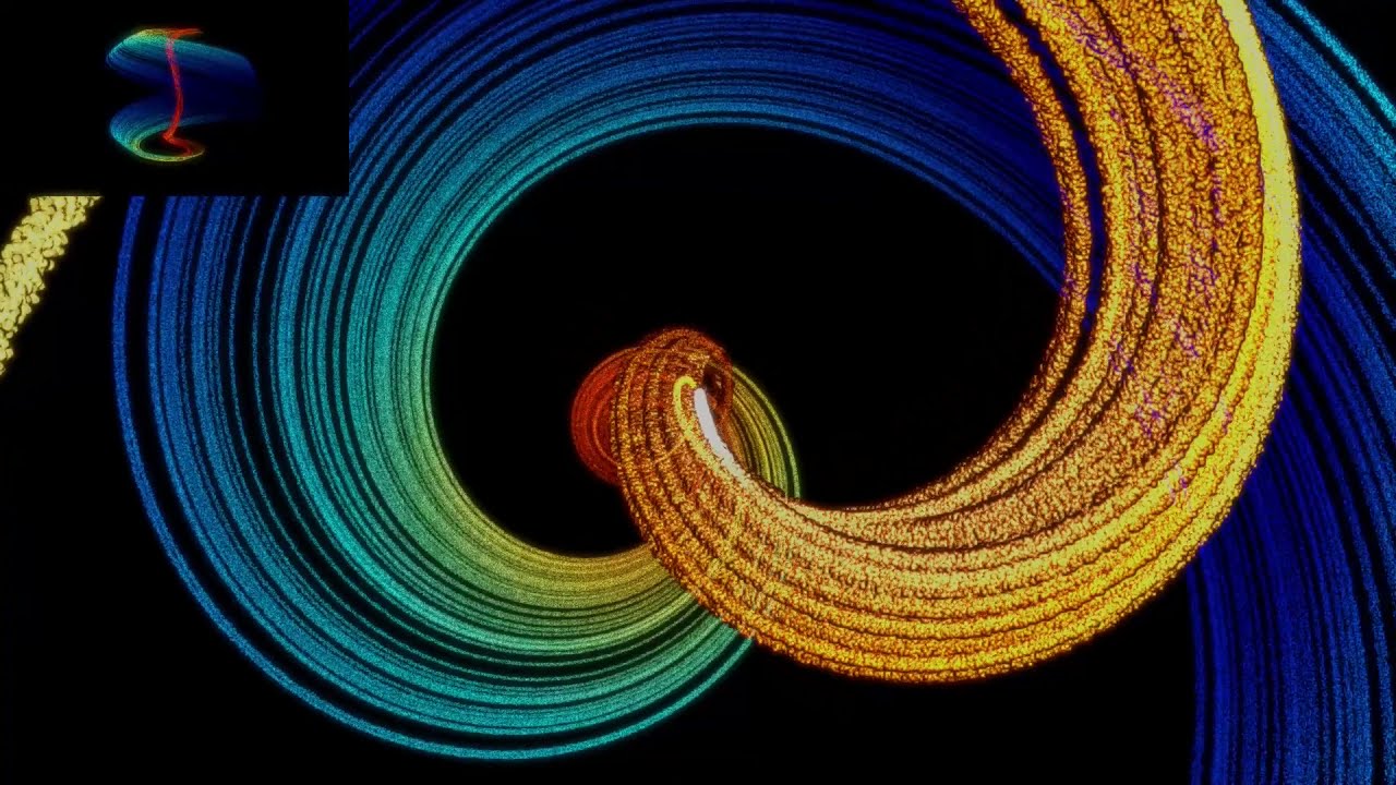









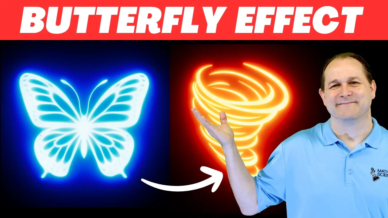

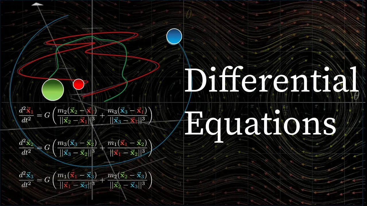
The Lorenz Attractor is a system of ordinary differential equations (dx/dt = σ(y-x), dy/dt = x(ρ-z)-y, dz/dt = xy-βz) that exhibits chaotic, nonlinear behavior where small changes in initial conditions produce vastly different outputs (the butterfly effect); this system can be visualized in 3D using Processing by implementing the equations with specific constants (σ=10, ρ=28, β=8/3), storing trajectory points in an array list, and drawing them with beginShape() and endShape() to connect the points.
Coding Challenge: Lorenz Attractor Visualization in Processing
Added:Basic understanding of ordinary differential equations (ODEs) and how they model rates of change mathematically.
Concepts of numerical integration, specifically Euler's method for approximating continuous equations using discrete time steps in code.
Familiarity with the Processing programming environment (Java-based), including setup, draw loops, and basic 3D rendering concepts.
Fundamental knowledge of 3D coordinate systems (X, Y, Z axes) and vector manipulation.
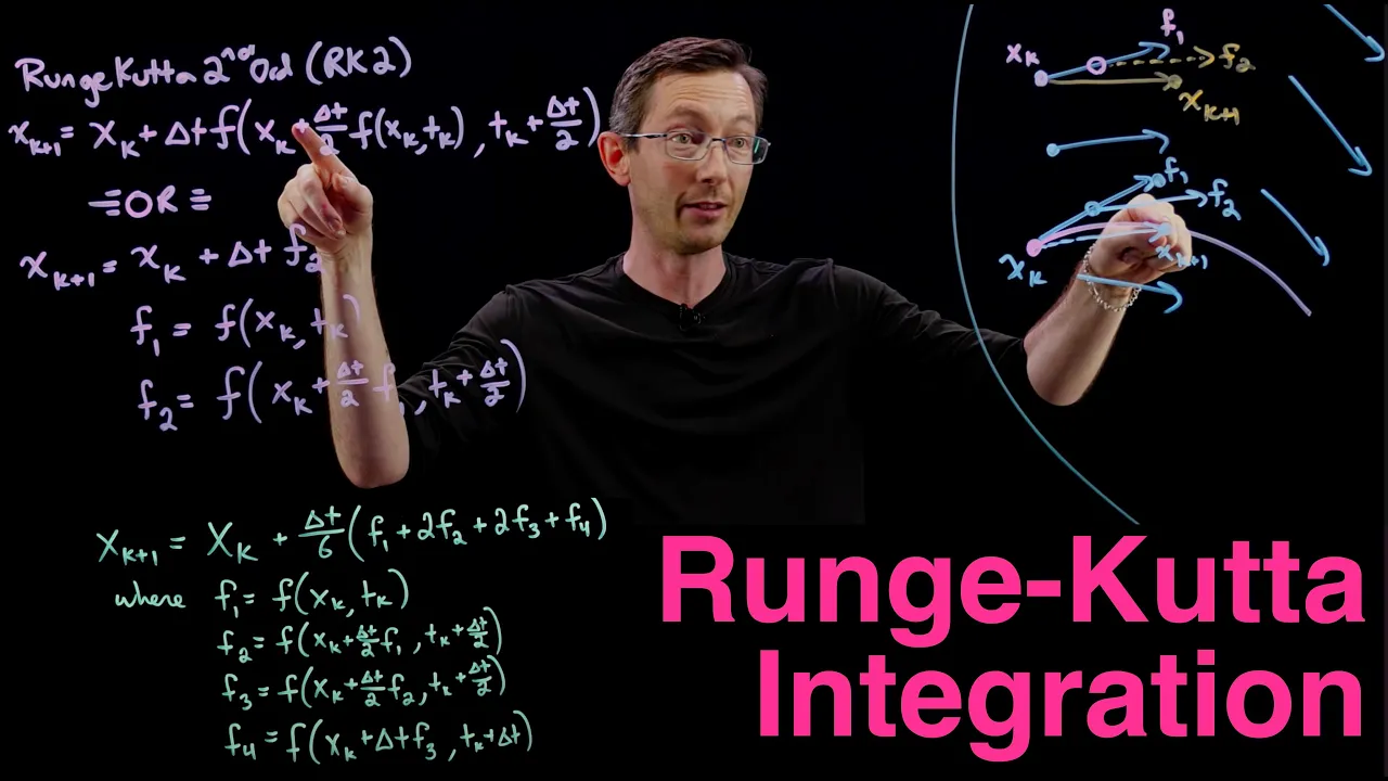
Implementation of more precise numerical integration techniques, such as the 4th-order Runge-Kutta (RK4) method, to reduce approximation errors.
Exploration and visualization of other famous chaotic systems, such as the Rössler attractor, the Aizawa attractor, or Clifford map fractals.
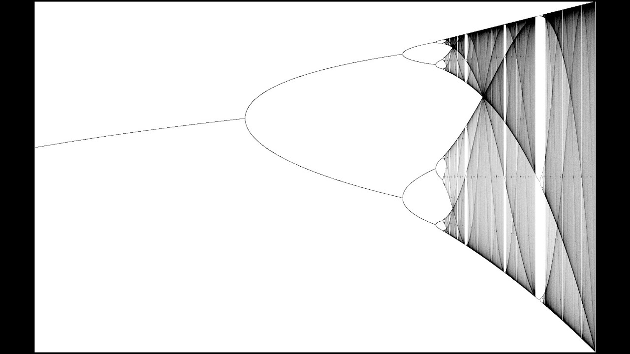
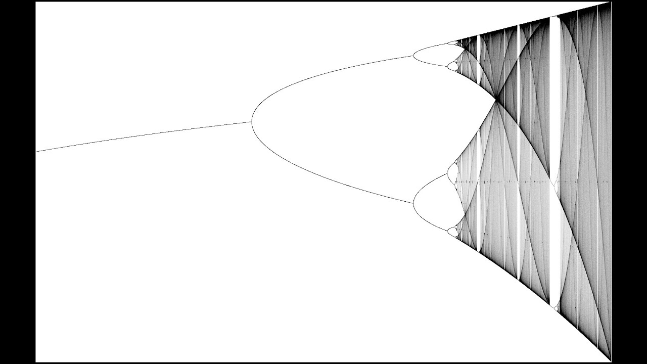
Constructing bifurcation diagrams to visualize and study how changing system parameters (such as the Rayleigh number) leads to stable, periodic, or chaotic behavior.
Leveraging GPU-accelerated particle systems and custom GLSL shaders to render and animate millions of points along the attractor path in real-time.
Studying the practical applications of chaos theory in weather forecasting, secure communications, cryptography, and fluid dynamics.
415.1K views8.9Klikes21:21Original Release: 2016-05-06
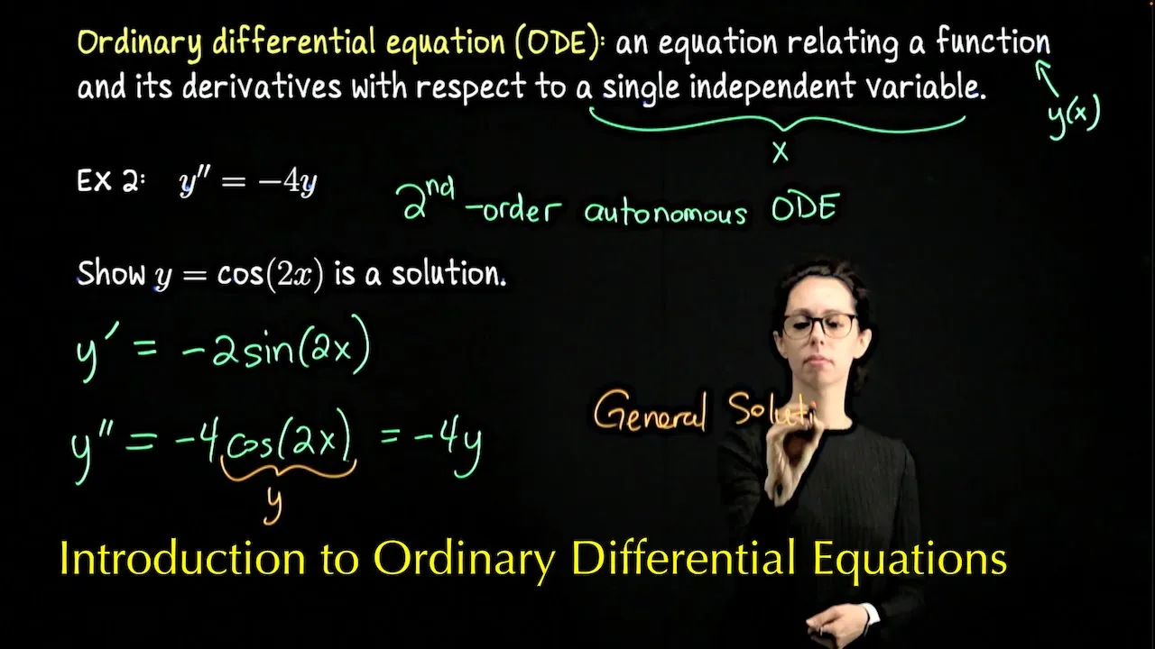
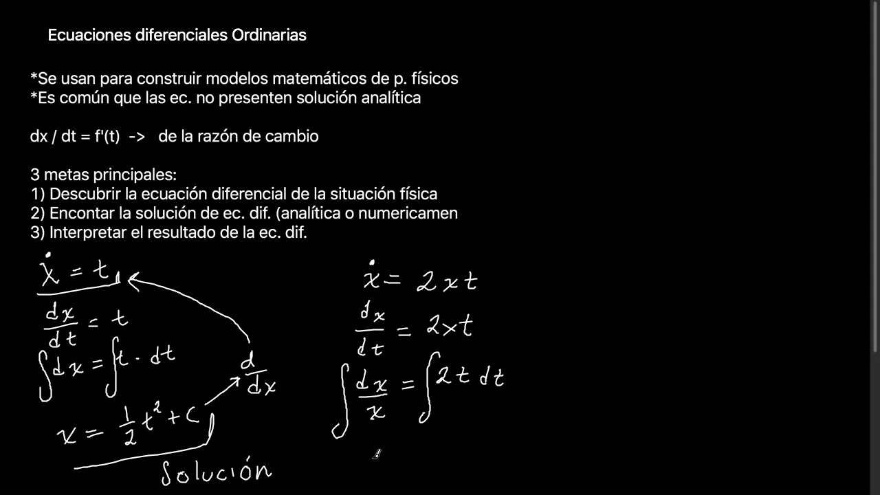
hello and welcome to another coding challenge in this coding challenge I am going to implement the system you see over here on the right called the lorenza tractor visualize that in 3D in processing all in one session here which will hopefully be about 10 to 20 minutes we'll see how long it takes I've got a timer running up there okay so before I start actually writing the code for it I want to talk about what this system is why does it exist why is it interesting and how does the math behind it work on a kind of um you know higher level and then we'll start looking at the formulas for it and implementing those formulas in code okay so the Loren system you know there's a lot of resources for this online I'm going to put a few in the description of this video Paul Bor site is a particularly useful one that I'll just mention really briefly but I'm going to look just at the Wikipedia page here which says the Lorent system is a system of ordinary differential equations okay so the first thing we have to tackle here is what is a differential equation I could easily I got a timer running here I could easily be here for like the rest of the day talking about differential equations and confusing myself over and over again but the basic idea of a differential equation is an equation that looks at how a certain variable changes according to other variables how the rate of change of a variable is affected by other variables in a system that rate of change being a differential so let me give you an actual practical real world example that might help solidify this understanding let's say you have a spring okay so I have a spring connected to a wall with a Bob at the bottom and you could think of this spring as having a position called y How does its y position change over time that's often written as the change in y over time you could think of that in programming speak as y equals y plus the change in y right every frame of Animation y changes but it changes based on it's uh the the rate of change of Y actually changes based on the Y position itself if you pull all the way down here how fast it's going to spring back is going to be much more than if you pull it over here so dy over DT the change in y the differential of Y is a function of other variables in the system itself y itself this is a differential equation and so you know this actually comes up all the time in programming you have position you have velocity velocity being the derivative the rate of change of position this is a something that you'll see over and over again and here the Loren system is defined by these particular differential equations the rate of change of X over time the rate of change of Y over time and the rate of change of Z over time now these variables X Y and Z those are those Define the state of the system but I'm going to use those literally as Xyz positions to visualize uh this particular to get this particular structure so if I look at those POs those those values the state XYZ over time and draw them with colors and lines I'm going to see this particular um this particular system so why is this system in interesting it turns out that the luren system which was um you know invented or discovered in 1963 by Edward Edward Edward Edward Edward Loren um you know he was studying meteorological conditions the flow of the atmosphere this type of thing it's one of these chaotic nonlinear systems meaning whatever the inputs you feed into the system uh um you feed some inputs into the system you calculate that system over time it's a deterministic system that will produce an exact result every time with the same inputs but if you change the input ever so slightly you could get a widely different output it's nonlinear a tiny change to the input makes a large change to the output this is the butterfly effect a little butterfly flaps its wings changing the air just a tiny bit in the uh outside on one side of the world and on the other side of World a giant volcano erupts okay so this is this idea of a nonlinear system it's chaotic it's unpredictable um and a lot of these types of systems exist in nature and this is one particular example of a model of that type of system okay so now let's look at these formula and let's try to figure out how we're going to actually make this happen in code I think we're ready so we know that I need three variables an x a y and a z so let me go to my uh program here and I'm going to close this one and I'm going to start start writing some code from scratch and I am going to give myself an X and A Y and a z and I'm going to give them some initial values uh like that okay so we're we're good so I solve those equations I know I need an x a y and a z so that's a good start now one thing I should mention really briefly as I'm four about five minutes into this is that notice I defined those values as floats if you look at examples you'll find on the internet often the the data type that will be used is a double a double being just like a floating Point number but having more decimal places and sometimes with these systems you really need a high degree of accuracy but I'm just some person here on the internet programming colors and things on the screen I don't care if it's a little bit not so accurate and Float is a bit more native to processing so I'm going to use floats um okay so now what I need to figure out is I want to kind of implement these equations so let's just start with x the change in X over time equals uh Sigma that's the Greek letter Sigma times y- x so first of all I I can't use the Greek letter Sigma easily in my code so Sigma I'm going to make a row I'm going to make B and beta I'm going to make C which I I realize is a bit confusing but that's what I'm going to do so those are constants by the way I need constants for those values so let me go back to my code and I'm going to say a float a equals 1 so I'm just going to start with the constant one now what I'm going to do is have this particular calculation happen over and over over time right it's supposed to happen over time time this is the interesting thing about this those formulas the change in X over time we're those formulas are talking about real life time that's continuous our time in processing is frame by frame by frame so every cycle through draw is one unit of time so what I'm going to say is that the change in x equals that constant time what y - x y - x and now X = X Plus that change in X it's really that simple right I'm just taking that exact formula that says the change in X over time equals the constant times y - x and now change in X just means change X by that value xal X Plus DX so I can actually start to go and Implement Y and Z the change in y and the change in Z and now I just need to go back and refer to those formulas again x * B minus zus y oh God I hope I get this right this is hard to do oh no sorry x x times B minus Z * y did I get this right minus y I want to have spaces there what's wrong here oh it doesn't know what B is I'll fix that later and now the change in Z is x * * y - c * Z so it's x * y - c * Z so this should be good and now I just need to get some spacing here and I need to also add uh two more constants float b equals 1 float Cals 1 and now I need to just change x y and z x y z x y z y z Dy DZ okay so this is the idea I Implement those formulas directly from the Wikipedia page to calculate the change in X the change in y the change is the and then actually change them now here's the thing what is my time there's a weird sort of thing that I'm going to bring up here which is my time step so right now every frame is like a singular unit of time but the the pattern that I'm going to draw right is going to look you know I'm not going to be able it's going to look something like this and in the sort of continuous world I was moving this marker continuously but in the processing animation world I have point point point point point so how close and I might connect those with a line so do I want to see my result look like this or do I want to see it as more continuous curve how fine do I want those to be and that's the sort of DT right if you think about oops I'm going to come back over here right really I'm saying DX over DT equals something so what I want to do is actually take that something something and multiply it by DT what is the change of time for each frame so what I'm going to do is also introduce a variable called DT and I'm going to say it's like 0 point I'm just going to make that one for right now but I'm going to take the whole thing and multiply that by DT for each one of these to sort of scale and I'll show you how different that's going to look um uh as we um as I continue doing this so now we've got those formulas implemented now we've got to see is anything working correctly here so I need a way of figuring that out the first way I'm going to do to figure that out is first just make sure I the program runs I'm going to add a black background and I'm going to run it and okay so I don't have any errors that's a good sign you know one thing I could do is I could say print line XYZ so I could sort of look at what's being printed out now notice something here all I'm doing is getting the values of zero so there's a little bit of an issue here which is that that doesn't make any sense so I can't start with 0 if I start with 00 these formulas are only ever going to produce 00 so I got to modify the inputs a little bit and I'll just start with X as like 0.01 that should do pretty well and if I run this again we should see look look I'm getting some interesting values there now what are these values producing anything of note not really but why not well because my constants I just made my constants one one and one so the Loren attractor Works a particular way based on what those input constants are so if I go back to the Wikipedia page I could sort of find um somewhere on here it's going to give me some values I could use like Sigma equal 10 rowal 28 and beta equal 8 / 3 so let's use those constants I believe Sigma was a b was um B was 28 and C was uh 8 divided 3 and I'm going to do that just to make sure I get a floating point value okay so I think that should should work I'm like skeptical and we should see o not a number okay so what have I done wrong here I might have to time out this video see how long this debugging takes and this might get edited out if it starts to take a really long time but let's look here um so what have I done wrong here uh XYZ um so let's let's comment out and just do X for a second uh and see what I get oops and I just want to look at X oh I had some numbers and then I got not a number for y so I might just be like one is a terrible number for DT because I'm like it's as if I'm teleporting myself Through Time massively fast so let me just make this 0.01 yeah okay this is more like what I expected to see Al those numbers are getting incredibly small I hope I implemented this right I have to check my formulas let's go back here and see if I'm getting some reasonable formulas okay good reason okay so this is better this is what I expected to see okay great so now I'm seeing some numbers that make more sense so my issue there was literally just having and think that won't get edited out was just having the number one it and it just sort of went off to Infinity super fast these systems um they don't have a recognizable repeating pattern and they tend towards they often tend towards infinity or some like non-existent value okay so let me go back to 0.01 now I want to be to figure out is something actually working here so the first thing I'm going to do is just say stroke 255 and I'm going to I'm also going to translate to the center of the window and I'm just going to draw a point and I'm just going to do this in 2D so I'm not going to worry about the Z I just want at least see like let me plot those the state of the system over time with XY so let's do that and ah good this is very good so it looks like I did the formulas correctly you can start to see like that's something there so I'm actually we're kind of like we're Trucking along here I've got the Loren system like sort of visualizing right now so that really basically I'm done however I want to make this look like something I want to make this look like a 3D shape I want to maybe add some color to it I want to be able to spin around it I want to I need to do more with it maybe I want to be able to like explode it so that all the points should like fly off of it and come back so I want to do even though in 13 minutes we kind of got the math down I want to do more with this in terms of the visual output of it so um so let's go forward with that so the first thing that I'll do is let's just go ahead and work in 3D so I'm going to change the renderer to p3d and then I'm going to add the Z point so we should see now that um it's the same it looks pretty similar but there's actually a z value there now one thing I want to add also is just I want to use the uh the processing uh function scale so scale is a transformation you can add to your scene to kind of like stretch it out a little bit might be to get this through zooming in and out as well but I just want all the points to be sort of spaced out a bit more and look a little bigger so I'm going to basically scale everything by five so we can see yeah so this looks so now I kind of have a bit of a closer view you can see all the points of Loren's tractor are being plotted in 3D now here's the thing how am I getting all these points on the screen I'm just drawing one point at a time well notice how my background is in setup so this worked just to see that the system was working but it's not going to be a very good solution for eventually over time being able to manipulate this system so what I need is some sort of data structure some sort of list that I can store all the points of the Lorenzo tractor so let me do that and what I'm going to do for that is an array list this is where we might rather be in JavaScript and I'll try to make a JavaScript version of this as well I'm going to call that points I'm going to make that a new empty array list so this is the syntax for something in Java called an array list which is a flexibly sized array something I could just add to and I'm calling it points and the data that I'm going to put into that array list are P Vector objects why do I want a p Vector object it's because every single frame I'm going to say points. add a new P Vector with that X Y and Z okay so I want to add a new Vector with X Y and Z to that particular array list and we can see that this is still working nothing is broken yet and what do I want to do now as those points are being added over time I want to draw all of them because I need to erase the background right so let let me just show you what I mean I'm going to move this background to draw this is actually going to produce kind of an interesting result because now you're going to see this point ah I kind of love this just moving along the pattern of the Lorenzo tractor it's kind of this beautiful interesting kind of chaotic motion I just want to stop and watch it but I'm 15 minutes in I want to see if we can wrap this up in about 20 minutes so I'm going to keep going so what I want to do is instead of just drawing the existing Point what I want to do is say for every vector v in that array list points draw a point at v.x v.y and v.z so I'm now saying instead of just drawing the current Point Loop through and this is known as an enhanced Loop in Java for every vector v in the array list points draw a point at VX v y v y v y back after a technical hiccup you can see that the entire Loren attract Vector is drawn with each element as a separate Point based on every B Vector that's in that array so really essentially I'm done there you go it's in 3D that's the entire Lorenzo tractor shape but I do want to add some more things to this and give you some exercises to think about what you might do with this so first let's just change the way we're drawing this a little bit um one thing that I could do is connect all the points with a line so instead of drawing everything as a single point I could actually set the vertex of a shape so if I say begin shape before I draw all the points and end shape after I draw all the points with vertex instead of Point what that's going to do is connect every point and you're going to see now that whoa it's doing it but it's actually trying to fill it in as if it's an entire shape so there might be some interesting things I could do with that but for now I'm just going to add no fill and we're going to be able to see now this continuous line so I could zoom into it and sort of see that every point is now connected right so now we have this continuous shape which is a nice start of sort of seeing how I could sort of Tinker with how this is visually I could also try to come up with like a clever way of changing the colors of it I'm sure that you as a wonderful person on the internet with visual design Talent will do something much more interesting but I'll just show you really quickly ah I already have that in there because I that was from the technical glitch but I could add something called color mode and I could change the color mode to HSB meaning Hue saturation brightness so what I could do is set the stroke of with a some sort of hue a saturation of 255 the maximum and a brightness of 255 so I'm now now as I draw it it's going to have a particular kind of like turquoisey greeny Hue and why not while I'm doing this um make a variable start it as Zero have that variable be the Hue and for every single vertex uh increase that by some value and then uh if it goes above 255 uh reset it back to zero and now I should get uh why not have a rainbow since this is coding rainbow uh a rainbow Loren tractor um pattern so you can see as the color is changing we've got kind of yellow red to Yellow to Orange and that sort of thing so really okay so the last thing I want to mention so what's interesting about what I'm doing with this particular strategy separate from the Lorenzo tractor um separate from the Lorenzo tractor um algorithm itself is the fact that every one of these points is saved in memory in that array so one thing I might just demonstrate to you is the fact that those points can be manipulable in real time so for example one thing I could do in processing is I could write a vector called offset uh and I could say p vector. Random 3D that's going to be give me just a random unit Vector of unit one um of length one pointed in a random Direction and I could add that offset to every single Vector in the Lorenz tractor now if I run this it's kind of going to go crazy because the unit of I've scaled up by five so you can see it's like sh shaking and jiggling like crazy so what I could do is maybe shrink that offset down quite a bit by you know make it 10% of the length of itself and you can see now if I zoom into it you can see how the points are kind of moving ever so slightly in space now I'm not suggesting that what I've done is a particularly magnificent result but what if you had all those points move along a sine wave or what if you have those points expand out and then come back to the original location or morph into another shape or fill in the blank of your interesting idea there so what I think I would like you to do now that you've seen how to program this lorenza tractor from scratch first you don't have to do anything you're just watching this video maybe you want to go outside and toss a frisbee around or eat some lunch which is what I kind of want to do right now because I'm feeling a little woozy but I think what would be interesting what I'd be excited for some of you watching this video to explore is what types of other how can you put your own design spin on this particular shape what happens if you start to manipulate the variables right here are the constants that I'm using make up your own constants look up on the Internet some other known constants for the lorenza tractor that produce other kinds of shapes what happens if you change the DT variable what can you mess around with these formulas and get something else can you go to Paul could you go to a site and find a different kind of attractor that's not the Loren one there's a sort of there's a lot of these under the sort of category of strange attractors so try to make your own version of this uh be creative play experiment don't worry too much and share with me your your results but this has been hopefully something you've enjoyed which is programming the lorenza tractor from scratch in processing in 3D thank you very much for watching I'm thrilled to have finished this because you might not know there was about a 45 minute audio problem I really hope the audio is working right now and this is actually the end of this video thanks for watching and I'll see you in the future in in another video goodbye
Up Next

10:24
The Lorenz Attractor: Chaos Theory & Differential Equations
@mitocw
32.6K views•2016-07-28

4:43
Elliptic Curve Cryptography Explained: ECC, ECDSA, ECDH
@PracticalNetworking
28.5K views•2024-10-21
22:35
Mathematics of Gradient Descent Explained | Machine Learning Tutorial
@TheCodingTrain
253.8K views•2017-06-05

6:00
The Mathematical Impossibility of Accurate World Maps
@Vox
23.3M views•2016-12-02
Related Study Plans & Knowledge Roadmaps
Structured learning paths in Mathematics
mathematics
Tensor Calculus: Vectors to Riemann Curvature
01Mathematical Foundations: Linear Algebra & Calculus
02Covectors, Dual Spaces, and Tensor Basics
03The Metric Tensor and Index Gymnastics
+ 2 more learning modules
40h5 modules
Explore Roadmap
mathematics
Gödel's Incompleteness: Logic, Proofs & Limits
01Introduction to Formal Systems & Hilbert's Dream
02Set Theory, Cardinality, and Cantor's Diagonal Argument
03Arithmetization and Gödel Numbering
+ 2 more learning modules
14h5 modules
Explore Roadmap
mathematics
Galois Theory: Fields, Groups & Solvability
01Foundations of Abstract Algebra: Groups & Fields
02Polynomials & Field Extensions
03Splitting Fields & Symmetries
+ 2 more learning modules
24h5 modules
Explore Roadmap
mathematics
Non-Euclidean Geometry: Models & Geodesics
01Euclid's Fifth Postulate and the Birth of New Geometries
02Hyperbolic Space and the Poincaré Disk Model
03Geodesics: Defining Straight Lines in Curved Spaces
+ 2 more learning modules
15h5 modules
Explore Roadmap