
























![Extended Kalman filter for nonlinear state estimation (basic theory outline) [moved to new channel]](https://i.ytimg.com/vi/ASQttsoHLq0/maxresdefault.jpg)


To analyze nonlinear autonomous systems, first find critical points by solving f(x,y)=0 and g(x,y)=0 simultaneously, then linearize the system at each critical point using the Jacobian matrix to approximate local behavior, and finally sketch trajectories by combining these local analyses to understand the global phase portrait; this method is demonstrated using the nonlinear pendulum example, where critical points represent equilibrium positions (stable at θ=0 and unstable at θ=π), and linearization reveals different dynamical behaviors such as spiral sinks and saddles that explain the pendulum's physical motion.
Nonlinear Systems and Pendulum Dynamics | MIT 18.03
Added:Fundamentals of Ordinary Differential Equations (ODEs), specifically second-order linear ODEs and autonomous systems.
Linear algebra concepts, including eigenvalues, eigenvectors, and solving systems of linear differential equations.
Multivariable calculus, specifically computing partial derivatives and constructing a Jacobian matrix.
The concept of Taylor series expansions for approximating nonlinear functions locally.
Basic Newtonian mechanics, particularly the rotational dynamics and forces acting on a simple damped pendulum.
Lyapunov stability theory and using energy methods (Lyapunov functions) to prove global stability of critical points.
Bifurcation theory to analyze how the qualitative behavior of nonlinear systems changes as physical parameters vary.
Limit cycles and the Poincaré-Bendixson Theorem for identifying isolated periodic orbits in two-dimensional state space.
Chaos theory and higher-dimensional nonlinear dynamics, such as the chaotic motion of a double pendulum or the Lorenz attractor.
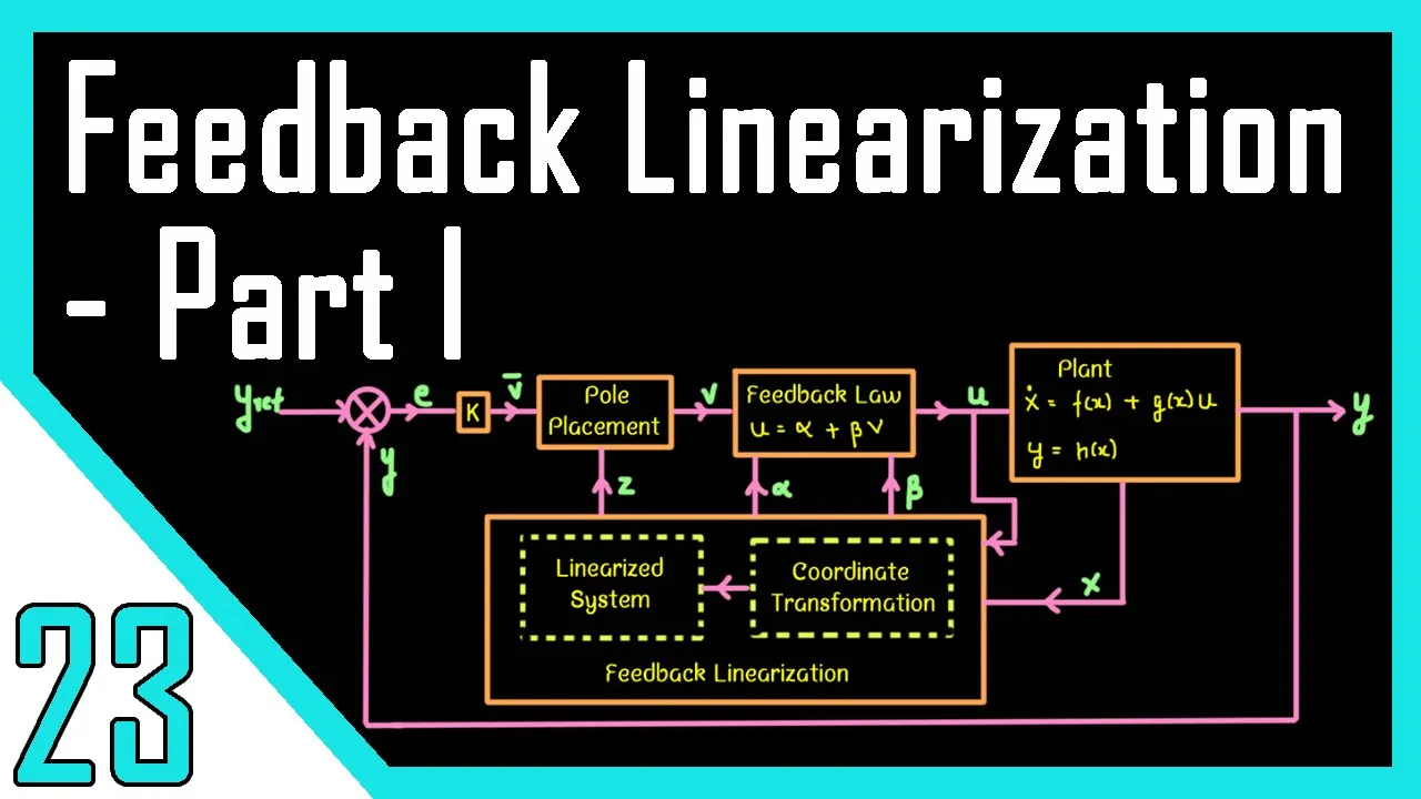
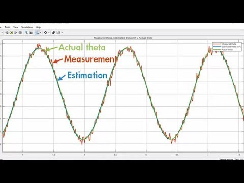
Nonlinear control systems design, including feedback linearization and state-estimation techniques like the Extended Kalman Filter.
71.8K views367likes47:11Original Release: 2008-01-17
So the topic for today is we have a system like the kind we have been studying, but there is now a difference.
A system of first order differential equations, just two of them. It is an autonomous system meaning, of course, that there is no t explicitly on the right-hand side. But what makes this different, now, is that it is nonlinear.
In other words, the functions on the right-hand side are no longer simple things like ax plus by, cx plus dy. Those are the kind we have been studying. But we are going to allow them to have quadratic terms, sines, cosines, different stuff there that are not linear functions anymore.
And the problem is, if it's a linear system you know how to get a sketch of its trajectories without using the computer by using eigenlines. You were very good at that on the exam on Friday. Most of you could do that very well. But what do you do if you have a nonlinear system? The problem is to sketch its trajectories.
In general, there are not analytic formulas for the solutions to nonlinear systems like that.
There are only computer-drawn things.
But sometimes you have to get qualitative information, a quick idea of how the trajectories look.
And, especially on Friday, I will give you examples of stuff that you can do that the computer cannot do very well at all. Okay, so the problem is to sketch those trajectories. Now, what I am going to do is -- The way I will give the lecture is, this is the general problem. We have to do two things sort of simultaneously. I will give a general explanation using x and y, but then, as we do each step of the process and talk about it in general, I would like to carry it out on a specific example. And so we will do it with a specific example. The example I am going to carry out is that of the nonlinear pendulum.
I am using this because it illustrates virtually everything. And, in addition, it has the great advantage that, since we know how a pendulum swings, we will be able to, when we get the answer, verify it and, at various stages of the procedure, verify that the mathematics is, in fact, in agreement with our physical intuition. It is going to be a lightly damped pendulum because I am going to have to put in numbers in order to do the calculations. And that seems like a good case which illustrates several types of behavior.
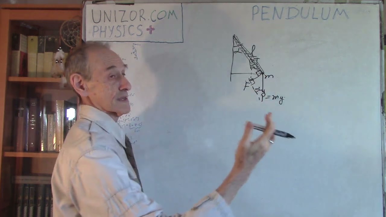
Let's first of all, before we talk in general, remind you of the pendulum. The pendulum I am talking about has the vertex from which it swings.
This is a rigid rod. It is not one of these string-type pendulums. There is a mass here.
The rigid rod is of length l. And so it swings in a circular orbit like that back and forth in a circle.
And let's put in the vertical distance, the vertical position rather. And now, as variables, of course normally we use neutral variables like x and y.
But here x and y are not relevant variables to describing the way the mass moves. The obviously relevant variable is theta, this angle. Now, I am taking it in the positive direction. Here theta is zero.
As it swings, theta becomes positive.
Over here, when it is horizontal, theta has the value pi over two and then so on it goes.
Values here correspond to negative values of theta.
That is how it swings. Now, just to remind you of the equation that this satisfies, it satisfies F equals ma, rather ma equals F. Now, the acceleration is along the circular path. And that is different from the angular acceleration. I have to put in the factor of the length. You had that a lot in 8.01 so I am simply going to write it down.
It is the mass. Therefore, the linear acceleration along the circular path is equal to the angular acceleration times l. It is l times theta prime prime, or double dot if you prefer.
And so this much of it is the acceleration vector.
Now, once the force is acting on it, well, there is a force of gravity which is pulling it straight down.
But, of course, that is not the relevant force.
I am interested in the force that acts along that circular line. And that will not be all of the pink line but only its component in that direction.
And the component, I fill out the little right triangle. And then the way to get the component in that direction, the vertical pink part has the magnitude mg. But, since I only want this part, I have to multiply by the sign of this angle.
Now, sometimes I have given on a diagnostic test to students when they enter to what angle is that?
But, of course, anybody can guess it must be theta. Otherwise, why would he be asking it? So this is still the angle theta. You can prove these two triangles are similar. One of them I haven't even written in, but it would be the right triangle whose leg is perpendicular to it. So the right angle is here.
If that is theta then the length of this small pink line is mg times the sine of theta.
That is the force due gravity. It is mg sine theta.
Except in what direction is it? It is acting in the negative direction. This is theta increasing.
This is the opposite direction, so I should put a negative sign in front of it. But that is not the only force.
There is also a damping force that goes with a velocity.
And that also occurs if the angular velocity is positive, the angle theta is increasing, in other words, the damping force resists that. It is opposite to the velocity.
So the velocity is going to be l times theta prime.
There is my velocity v. Linear velocity, not angular velocity. And so this is going to be a negative times some constant times that c1.
Now, that is the equation. But let's make it look a little better by getting rid of some of these constants.
If I write it out this way and put everything on the left-hand side, the way it is usually done in writing a second order differential equation. Theta I am going to divide through by ml and put everything on the left-hand side and in the right order. Next should come the theta prime term. And so that is going to be c1l divided by ml, so that is c1 over m.
The l's cancel out. And, finally, the last term on the right, I will move this over to the left, but remember everything is being divided by ml, so the m's cancel out, and it is plus g over l times the sine of theta. That is our differential equation. But let's make it look still a little bit better by lumping these constants and giving them new names. It is going to be finally theta double prime. I will simply call this thing the damping constant. I will lump those two together into single damping constant. And then g over l, I will lump those together, too.
And we usually call that k. It is k sine theta.
Now, this is a second-order different equation, but it is not linear.
If this were a month and a half ago and I said solve that, you would stare at me. But, anyway, you couldn't solve that. And nobody can, in some sense. It is a nonlinear equation.
It doesn't have any exact solution.
The only thing you could do is look for a solution in infinite series or something like that. Well, what do you do?
You throw it on the computer, that is the easy answer, but what does the computer do? Well, the first thing the computer does is turns it into a system because the computer is going to use numerical methods to solve it.
But only those methods, the formulas it uses, Euler or modified or improved Euler or the Runge-Cutta method, they are always expressed not for single higher-order equations, but instead they always assume that the equation has been converted to a first order system.
Let's do that for the computer, even though it will do it itself if nobody tells it not to.
Theta prime is equal to, now I have to figure out what new variable to introduce. Normally we use x prime and call that y. That really doesn't seem to be very suitable here. But what do the physicists call it? This is the angular velocity.
And the standard designation for that is omega.
Two Greek letters. I told you this was going to be hard. Omega prime equals what?
Well, omega prime equals, now you do it in the standard way, you convert the system, but remember you have to put the theta first. So it is minus k sine theta.
The theta first and then the omega term first. So minus c times omega, minus c theta prime, but theta prime is, in real life, omega.
And now we have our acceptable system.
The only problem is I have not put in any numbers yet.
The numbers I am going to put in will make it lightly damped.
I am going to give c, think of it here, this is the damping, and this is the stuff representing, well, if I want to make it lightly damped all I am saying is that c should be small compared with k, but it doesn't have to be very small. I am going to take c equal one and k equal two, and that will make it lightly enough damped. This is the lightly damped value, values which give underdamping.
In other words, they are going to allow the pendulum to swing back and forth instead of strictly going ug and ending up there. Finally, therefore, the system that we are going to calculate is where theta prime equals omega and omega prime equals negative two sine theta minus omega.
And now what do we do with that?
There is our example. That is our system that represents a pendulum swinging back and forth, damped away. And now let's go back to the general theory. And, in general, if you have a nonlinear system, how do you go about analyzing it?
The first step is to find the simplest possible solutions, solutions that you hope can be found by inspection.
Now, what would they be? They are the solutions that consist of a single point. How could a solution be a single point? Well, like the origin for a linear system, those points which form solutions all by themselves are called the critical points.
I am looking for the critical points of the system.
That is the first step. The definition is a critical point x zero, y zero.
For that to be a critical point means that it makes the right-hand side zero.
The f is zero there, and the g is zero there.
See the significance of that? If you have such a point, let's say there is a critical point, what is the velocity field at that point? Well, it is given by the vectors on the right-hand side, but the components are zero.
That means, at this point the velocity vector is zero.
Well, that means if a solution starts there, you put the mouse there and tell it to move, where do you go? It has no reason to go anywhere since the velocity vector is zero there.
So it sits there for all time. And indeed it solves the system, doesn't it? It makes the right-hand side zero and it makes the left-hand side zero because x equals x zero, y equals y zero for all time. If that is true for all time it sits there then the derivatives, with respect to time are zero, so the left-hand sides are zero, the right-hand sides are zero and everybody is happy. Well, these are great points.
How do I find them? Well, by looking for points that make these two functions zero.
I find them by solving simultaneously the equations f of (x, y) equals zero and g of (x, y) equals zero.
A pair of equations. But the trouble is those are not linear equations. Linear equations you know how to solve, but they are not linear equations.
They are nonlinear equations that you don't know how to solve. And, to some extent, nobody else does either. There are very fat books in the library whose topic is how to solve just a pair of equations, f of (x, y) equals zero, g of (x, y) equals zero.
And it is quite a hard problem. It is even a hard problem by computer. Because, if you know approximately where the solution is going to be, you can make up the little screen and then the computer will find it for you. Or, even without a screen, it will calculate it by Newton's method or something else, it will zero in. The problem is, if you don't know in advance roughly where the critical point is that you are looking for, there are a lot of numbers.
They go to infinity that way and infinity that way.
In general, it is almost an impossible problem.
The only thing that makes it possible is that these problems always come from the real world and one has some physical feeling, one hopes, for where the critical point is. I am going to assume breezily and cheerily we can solve those. And I am only going to give you examples where it is possible to solve them.
But even there, you have to watch out.
There is a certain trickiness that will be talked about in the recitations tomorrow. Okay, so we found the critical points. Let's do it for our example.
Let's find the critical point. What is the pair of equations we have to solve? We have to solve the equations omega equals zero, minus two sine theta minus omega equals zero.
Now, it is not always this easy.
But the solution is omega is zero.
If omega is zero, then sine theta is zero, and sine theta is zero at the integral multiples of pi. The critical points are omega is always zero and theta is zero, or it could be plus or minus pi, plus or minus two pi and so on.
In other words, there are an infinity of critical points. That seems a little discouraging. On the other hand, there are really only two. There are really physically only two because omega equals zero means the mass is not moving. The angular velocity is zero, so it is only the theta position which is changing.
Now, what are the possible theta positions?
Well, here is our nonlinear pendulum.
Here is the critical point, theta equals zero, omega equals zero. Theta equals zero means the rod is vertical. Omega equals zero means that it is not moving, despite the fact that it is moving. Theoretically it is not moving.
Now, what is the other one? Well, there is theta equals pi.
Theta is now, starting from zero and increasing, I hope, through positive theta.
And when it gets to pi, it is sticking straight up in the air. And so the claim is that another critical point is theta equals pi and omega equals zero.
In other words, if it gets to this position, it starts out in this position and stays there for all time, as you see. [LAUGHTER] But my point is what about negative pi? That is the same as pi.
Two pi is the same as zero. So physically there really are only two critical points, this one and that one.
And they obviously have something very different about them. This critical point is stable.
If I start near there, I approach that critical point in infinite time. This one, if I start near there, I do not stay near there. I always leave it.
Of the two critical points, physically it is clear that the critical point is zero, zero and the other guys that look like it, two pi zero and so on is a stable critical point. Whereas, pi zero, when theta is sticking straight up in the air, is unstable. Now, of course, we will want to see that mathematically also, but basically there are just physically two point.
There are just two critical points.
Well, that raises the question what about all the others?
As you will see, we have to have those.
They are an essential part of the problem.
They are not just redundant baggage that is trailing along.
They are really important. But you will see that when we talk about finally how the trajectories look and how the solutions look. Now what do we do?
Well, we found the critical points, and now the work begins.
Virtually all the work is in this next step.
What do we do? Step two.
I can only describe it in general terms, but here is what you do. For each critical point x zero, y zero, a procedure that has to be done at each one, you linearize the system near that point.
In other words, you may find a linear system, the good kind, the kind you know about, which is a good approximation to the nonlinear system at that critical point. Plot the trajectories of this linearized system. And you do that near the critical point.
How do you plot the trajectories?
Well, that you knew how to do on Friday so I am assuming you still know how to do it on Monday.
In other words, if the system is linear you know how to plot the trajectories of it by calculating eigenvalues and eigenvectors and maybe the direction of motion if it is a spiral.
I will give you a couple of examples of that when we work out the pendulum. But, on the other hand, how do I line arise a system? Well, there are two methods.
There is one method the book gives you, which by and large I do not want you to use, although I will give you an example of it now. I want you to use another method because it is much faster.
Especially if you have to handle several critical points it is much, much faster. Let's first carry this out on an easy case, and then I will show you how to do it in general. Just this once I will use the book's method because I think it is the method which would naturally occur to you. Let's linearize this example at the point zero, zero.
What should be the linearized system?
In other words, it's only the nonlinear terms I have to worry about. Well, the minus omega is fine.
It is that stupid sine theta that I don't like.
But if theta is small, in other words, if I stay near zero, I could replace sine theta by theta. The linearized system is minus two. You replace sine theta by theta, since sine theta is approximately theta if theta is small, if theta is near zero. It is the first term of its Taylor series you can think of, or it's just the linear approximation starts out sine theta equals theta.
That is it. Or, you draw a picture.
I don't know. There are a millions of ways to do it. So we have it.
Now what do I do? Okay, now we will plot that.
The matrix, let's do our little routine, in other words.
I am writing right to left for no reason.
The matrix is, now I am just going to make marks on a board the way you did on your exam, zero, one. [LAUGHTER] I don't know what I am doing, but you know. Negative two, negative one, and then I write down the eigen-whatchamacallits. Lambda squared, plus lambda, minus the trace.
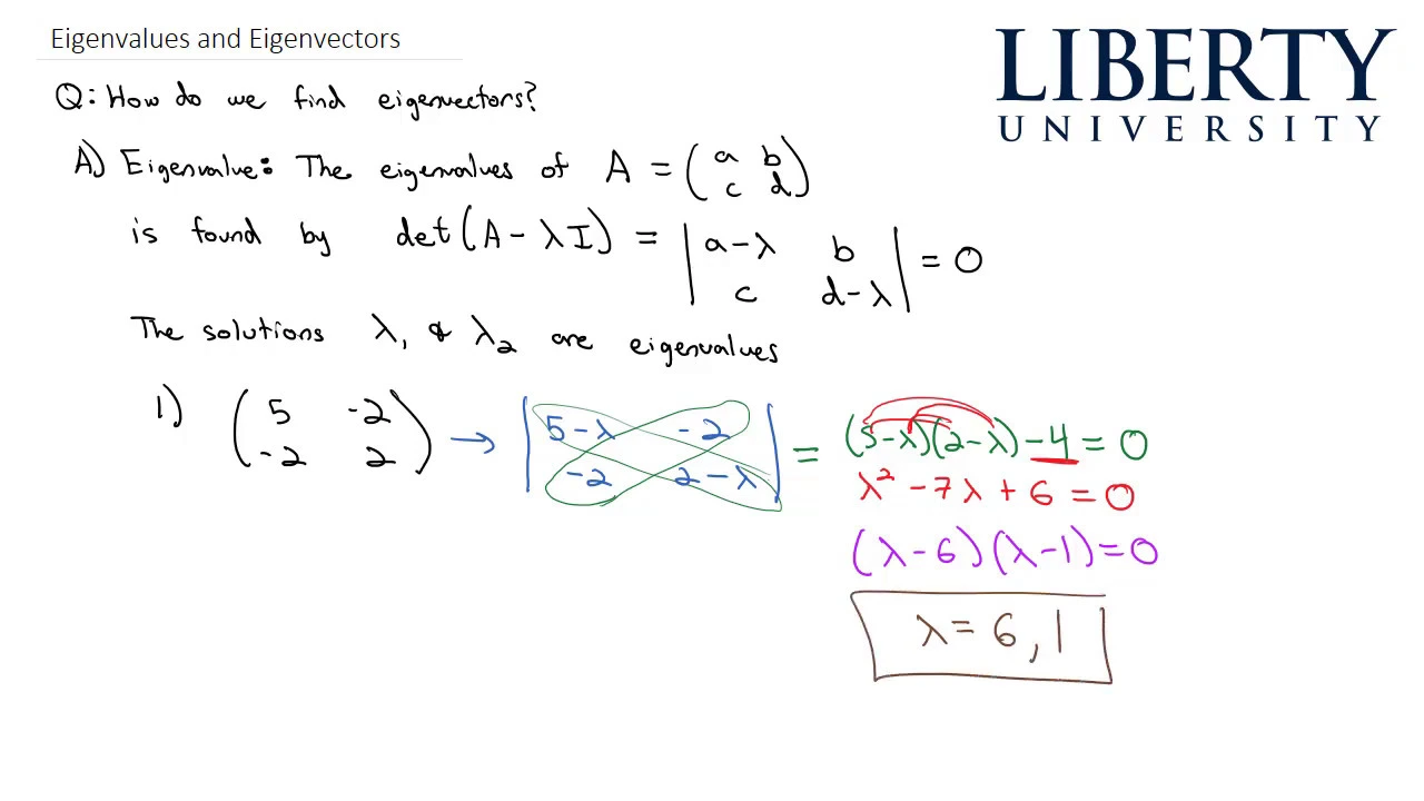
The determinant is minus, minus two, so it is plus two equals zero. And then, since it doesn't occur to me how to factor this, I will use the quadratic formula. It is negative one plus or minus the square root of, b squared minus 4ac, minus seven. Complex.
That means it is going to be a spiral.
I am going to get a spiral. Will it be a source or a sink since they are complex roots? Complex eigenvalues give a spiral. A source or a sink?
I tell that from the sine of the real part.
The real part is negative one-half.
Therefore, the amplitude is shrinking like e to the minus t over two. And, therefore, the spiral is coming into the origin.
It is a spiral sink since lambda equals minus one-half plus some number times i. Spiral sink.
And the other thing to determine is its direction of motion, which will be what? I determine its direction of motion by putting in a single vector from the velocity field.
Here it is. The vector at one, zero will be the same as the first column of the matrix. So that is zero, negative two.
Here is a vector from the velocity field, and that shows that the motion is clockwise and is spiraling into the origin. That is a picture, therefore, at the origin of how that looks.
Now, it is of the utmost importance for your understanding of what comes now that you understand in what sense this picture corresponds to the physical behavior of the pendulum. Let's start it over here.
What is it doing? That means that theta is some number like one, for example.
Let's make it smaller. Let's say a little bit.
And this is the omega access. If it starts over here that means the angular velocity is zero and theta is a small positive number. Theta is a small positive number. The angular velocity is zero.
It's velocity zero, theta small and positive.
I release it and it does that. What does this have to do with the spiral? Well, the spiral is exactly a mathematical picture of this motion.
What happens? Theta starts to decrease.
And the angular velocity increases but in the negative direction. This is negative angular velocity. Theta is decreasing.
The angular velocity gets bigger and bigger.
And it is biggest, most negative when theta is zero. It has reached the vertical position is when the angular velocity is biggest.
It continues then. Theta gets negative, but the angular velocity then decreases to zero.
Now the angular velocity is zero and theta is at its most negative, and then it reverses. Angular velocity gets positive as theta increases again, and so on.
These represent the successive swings back and forth.
Notice the fact that it is damped is reflected in the fact that each successive swing, the biggest that theta gets is a little less than it was before.
In other words, this point is not quite as far out as that one. And this one isn't as far out as that one. In other words, it is spiraling in.
Well, I hope that is clear because we now have to go to the next critical point. And now we have a little problem. If I want to do the next critical point, so what I want to do now is, in other words, I want to linearize at the point pi zero where theta is pi and the thing is sticking up in the air. The question is, how am I going to do that? This trick of replacing sine theta by theta, that doesn't work at pi.
That works at zero.
Now we have to go to the next step of the method.
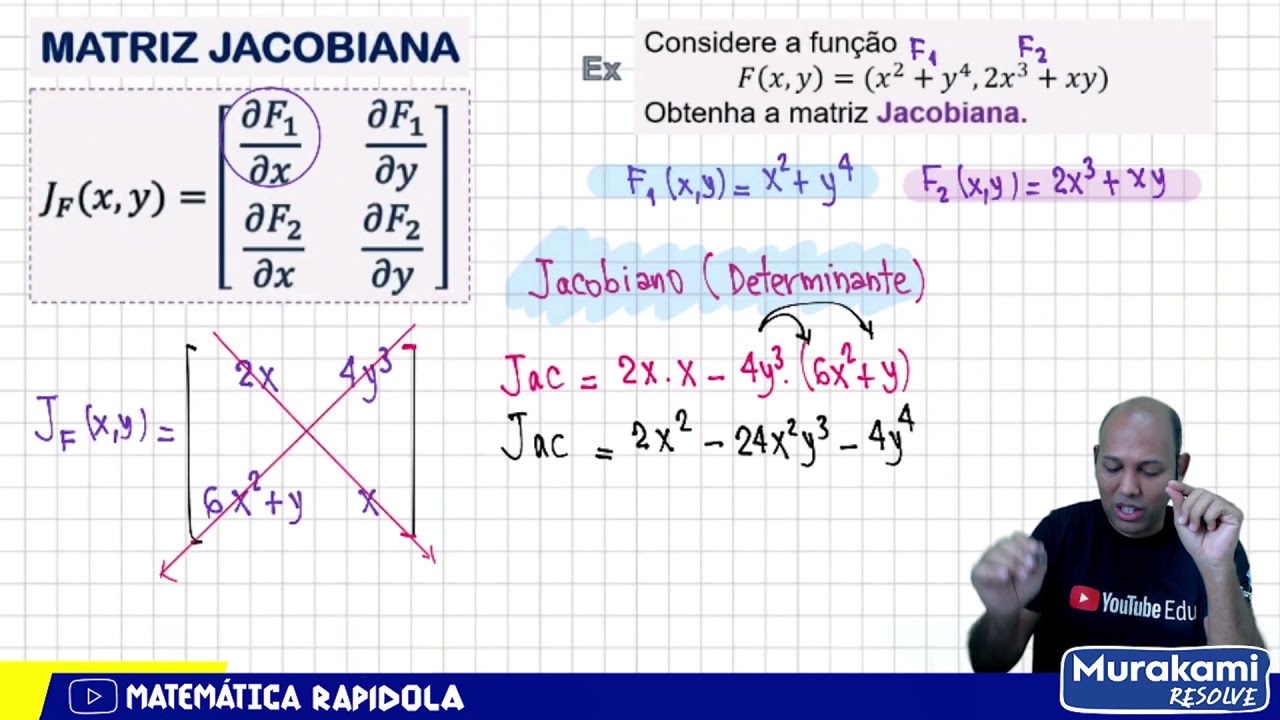
The way to do this, in general, as you will read in the notes because, as I say, this is not in the book, is to calculate the Jacobian.
I mean the Jacobian matrix. The Jacobian is the determinant. I mean, before you put the two bars down and made a determinant, you called it just the Jacobian matrix. And the formula for it is, it is calculated from f and g. The top line is the partial of f with respect to x and y, and the bottom line is the partial of g with respect to x and y.
So that is the Jacobian matrix.
I hope I get a chance at the end of the period to explain to you why, but I am most anxious right now to at least get you familiar with the algorithm, how to do it.
The notes describe the y of it, if we don't get a chance to get to it, but I hope we will. What do you do?
The Jacobian matrix. You calculate it at the point x zero, y zero.
I will indicate that by putting a subscript zero on it.
This means without the subscript zero it is the Jacobian matrix calculated out of those four partial derivatives. When I put a subscript zero, I mean I evaluated it at the critical point by plugging in each entry as a function of x and y.
You plug in for x equals x zero, y equals y zero, and you get a numerical matrix.
That is the matrix which is the matrix of the linearized system.
This is the matrix of the linearized system.
Trust me, it is. Now, since I don't expect you to trust me, let's calculate it. Here, we got the matrix another way, by this procedure of saying sine theta is theta-- What would we have gotten if we had done it instead by the linearized system? Let's do it that way.
Let's do it via the Jacobian.
I need to know the Jacobian of the system, which I have conveniently covered up. There is the system.
The Jacobian matrix is what? The top line, I take the partial derivative of omega first with respect to theta and then with respect to omega.
I then take the second line on the right-hand side.
I take its partial with respect to theta first.
That is negative two cosine theta.
And, thinking ahead, I erase the one and move it over a little bit. And what is the partial of that thing with respect to omega? It is negative one.
Does everyone see how I calculated that Jacobian matrix?
And now I want to evaluate it. Let's do our old case first.
At zero, zero what would this have amounted to? This would have given me zero, one. The cosine of theta at zero is one, so this is negative two, negative one.
I'm screwed. [LAUGHTER] That is the same as that. Now you see it, now you don't. We got our old answer back.
That should give us enough confidence to use it in the new case, where I don't have an old answer to compare it with.
What is it going to be at pi, zero?
The answer is J zero is now going to be -- Well, everything is the same. Zero, one, negative one.
And here cosine of pi is negative one, so negative two times negative one is two.
Everything is the same, except there is a two there now instead of negative two. Lambda squared plus lambda, the determinant, is now negative two.
And this factors into lambda plus two times lambda minus one.
So lambda equals one. The corresponding eigenvector.
I subtract one here, so the equation is minus a1 plus a2 is zero.
The solution is one, one, e to the t.
And for the other one, it's lambda is equal to negative two. This is the sort of stuff you can do, so I am doing it fast. Zero minus negative two is two.
So the equation is 2a1 plus a2 equals zero.
And the solution is now, I give a1 the value one, a2 will be negative two, and that is times e to the minus 2t.
Well, what does the thing then actually look like?
What I am now going to do is, I drew a picture before, that spiral picture we had before of the way the thing looked at the point zero, zero.
So at the point pi, zero how does it look, now? Well, it looks like the origin, but I am thinking of it really as the point pi, zero. In other words, I am thinking of a linear variable change sliding along the axis so that the point pi, zero now looks like the origin. If I do that then those two basic solutions, there is the one, one solution which is going out that way.
And it is going out this way. But the other guy is coming in along the vector one, negative two.
So one, negative two looks like this.
This guy is coming in at a somewhat sharper angle, coming in because it is e to the negative 2t.
And we recognize this, of course, as a saddle.
And I would complete the trajectories by putting in some of the typical saddle lines like that.
Now, I say that, too, gives a picture of what is happening to the pendulum near that point.
Let's, for example, look here.
What is happening here? This is theta, or really it is theta minus pi, is this axis.
In other words, this will be zero.
When theta is pi this will correspond to the point zero.
Here is omega. What is theta doing?
Starting up there this represents a value of theta a little bit less than pi, a little bit to the negative.
A little bit less than pi. Here is pi, so a little bit less than pi is over here. A little bit less than pi.
A little bit less. And omega is zero.
What happened? Theta started decreasing ever more rapidly so that the omega was zero here, now omega is negative and gets much more negative.
In other words, both theta decreases from that point and omega decreases also. What happened here?
Here, theta is a little bit more than pi.
Now it is a little bit more than pi.
Theta now increases until it gets to 2pi and then oscillates around 2pi. So theta increases.
And omega increases, too, because the angular velocity started at zero but, as theta gets more positive, omega gets positive, too, because theta is increasing. So omega increases and theta increases and it goes off like that.
Well, the final step is to put them all together to be the big picture. Here we are for three, let's say, the big picture. Plot trajectories around each critical point and then add some.
It's that last step that can cause you a little grief, but we will see how it works out.
Add some more, according to your best judgment. Let's make a big picture now of our pendulum the way it apparently ought to look.
Nice big axis since we are going to accommodate a lot of critical points here. Let's put in some critical points. Here is the origin.
And now here is the one at pi, let's say, here is one at 2pi.
I am going to add some of these others, 3pi, 4pi.
I won't in their values. You can figure out what I mean.
Zero here. And then here it will be negative pi, and here negative 2pi.
I guess I can stop there. That is the theta axis, and here is the omega axis. And now, at each one of these, I stay nearby and I draw the linear trajectories, the trajectories of the corresponding linearized system.
We decided here that the spiral went clockwise.
Now, this point is physically, of course, the same as that one. But mathematically, the Jacobian matrix is the same also because if theta is 2pi the cosine of 2pi is also one. And this is the same matrix.
So the analysis is identical. And, therefore, this point will also correspond to a counterclockwise spiral, as will this one. I am sorry, a clockwise spiral.
Here, too, all of these points are the same.
The behavior near them, clockwise spirals everywhere.
How about the other ones? Well, the other ones correspond to these saddles, so let's draw them efficiently by doing the same thing on every one, mass production of saddles.
There. And these guys go out.
And the other guys come in, etc. And so here we have a little bit there, a little here, here, there, everywhere, etc. Now what? Now you pray for inspiration.
And what you have to do is add trajectories that are compatible with the ones you have. Let's start with this guy.
Where is it going? Well, a trajectory either goes off to infinity, but generally they get trapped around critical points. This guy must be surely doing this. How about this one?
Yeah, sure. How about this one?
Why not? How about that one?
Yeah. But notice you are in trouble when two arrows you want to put in are near each other and going in opposite directions. That you cannot have.
Continuity forbids it. But notice if I, for example, had gotten these eigenlines wrong, if I made this come in and those go out because I made a simple error in drawing the thing, I would have said but I cannot draw this picture because this spiral wants to go that way but this, right next to it, wants to go the other way.
That is the way you would know if you made a mistake.
If you didn't make a mistake you won't have any trouble filling these things out. The directions of motions of the spirals, everything will be compatible.
Okay. What is this guy doing?
Oh, well, it must be joining up with that.
How about this one? Well, it must be coming back there. How about this one?
Well, trajectories cannot cross.
This guy cannot cross so it must be doing this.
All right. What is that trajectory?
Starts zero. Omega, on the other hand, is big and positive. Omega big and positive.
[LAUGHTER] I am scared. Omega starts.
Theta is zero. Omega big and positive.
It went around, slowed up, but continued beyond pi. And, in fact, went too far. It continued to go here and then finally wound around that one.
Now do you see why we had to have all the critical points?
You have to have all the critical points.
And not just the two physicals ones because the other critical points are necessary to describe a complicated motion that goes round and round and round until finally it crashes.
You are going to practice drawing these pictures and interpreting them in recitation tomorrow.
Up Next
11:55
Lyapunov Exponents Explained: Stability & Chaos in Difference Equations
@YunWilliamYu
188 views•2021-02-08

4:43
Elliptic Curve Cryptography Explained: ECC, ECDSA, ECDH
@PracticalNetworking
28.5K views•2024-10-21

20:22
Cantor's Theorem: Proof & Diagonal Argument | MIT 6.042J
@mitocw
33.1K views•2016-09-12

6:00
The Mathematical Impossibility of Accurate World Maps
@Vox
23.3M views•2016-12-02
Related Study Plans & Knowledge Roadmaps
Structured learning paths in Mathematics
mathematics
Tensor Calculus: Vectors to Riemann Curvature
01Mathematical Foundations: Linear Algebra & Calculus
02Covectors, Dual Spaces, and Tensor Basics
03The Metric Tensor and Index Gymnastics
+ 2 more learning modules
40h5 modules
Explore Roadmap
mathematics
Gödel's Incompleteness: Logic, Proofs & Limits
01Introduction to Formal Systems & Hilbert's Dream
02Set Theory, Cardinality, and Cantor's Diagonal Argument
03Arithmetization and Gödel Numbering
+ 2 more learning modules
14h5 modules
Explore Roadmap
mathematics
Galois Theory: Fields, Groups & Solvability
01Foundations of Abstract Algebra: Groups & Fields
02Polynomials & Field Extensions
03Splitting Fields & Symmetries
+ 2 more learning modules
24h5 modules
Explore Roadmap
mathematics
Non-Euclidean Geometry: Models & Geodesics
01Euclid's Fifth Postulate and the Birth of New Geometries
02Hyperbolic Space and the Poincaré Disk Model
03Geodesics: Defining Straight Lines in Curved Spaces
+ 2 more learning modules
15h5 modules
Explore Roadmap