

![[프로세싱 기초] 기본 도형들을 그려봅시다 (Processing basic drawing)](https://i.ytimg.com/vi_webp/TTqnlR3oWXk/maxresdefault.webp)






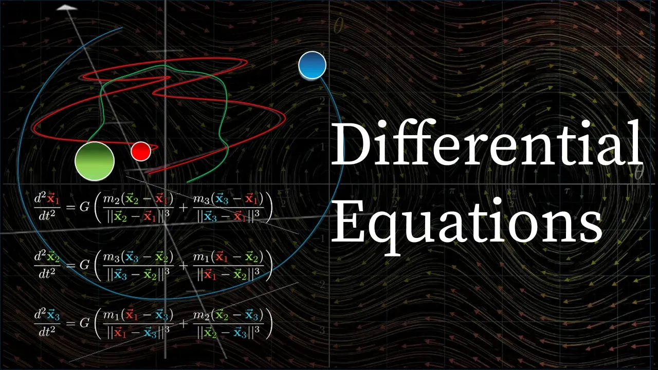












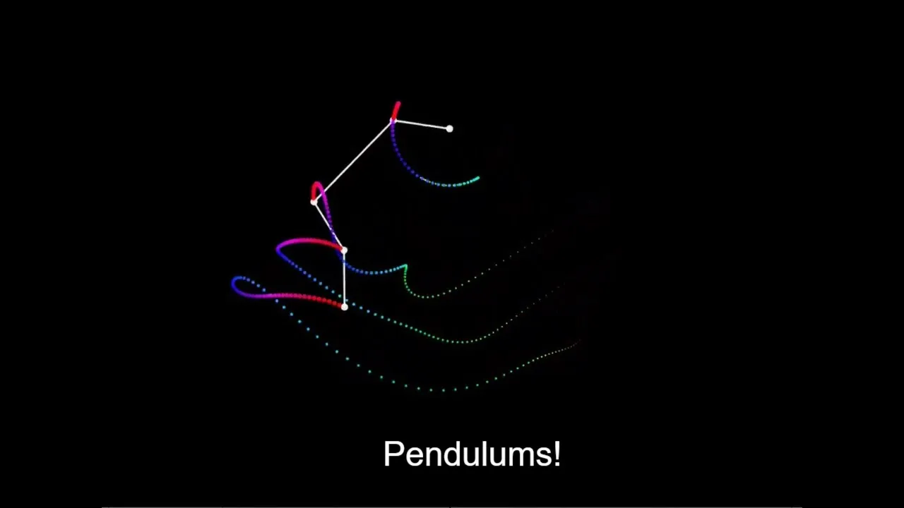

A double pendulum simulation can be created by implementing the angular acceleration formulas derived from Newtonian mechanics, which involve calculating the accelerations of both angles based on their respective masses, lengths, gravitational forces, and relative positions; this chaotic system produces complex, unpredictable trajectories that can be visualized using computer graphics.
Double Pendulum Simulation in Processing: A Step-by-Step Coding Challenge
Added:Fundamentals of the Processing programming environment, including the canvas coordinate system, the draw loop, and basic vector math.
Basic physics of a simple gravity pendulum, specifically angular displacement, angular velocity, and angular acceleration.
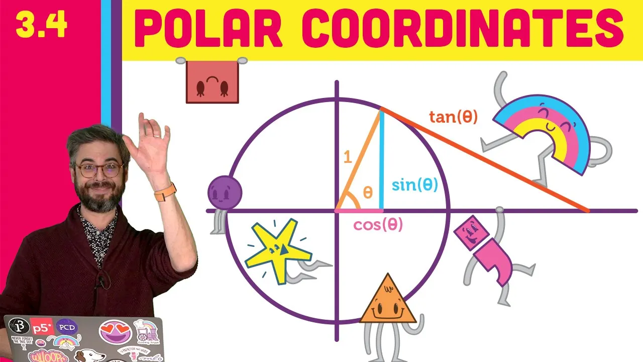
Trigonometric functions (sine and cosine) used for converting polar coordinates to Cartesian coordinates for rendering.
Introductory numerical integration concepts, such as Euler's method for updating state variables over discrete time steps.
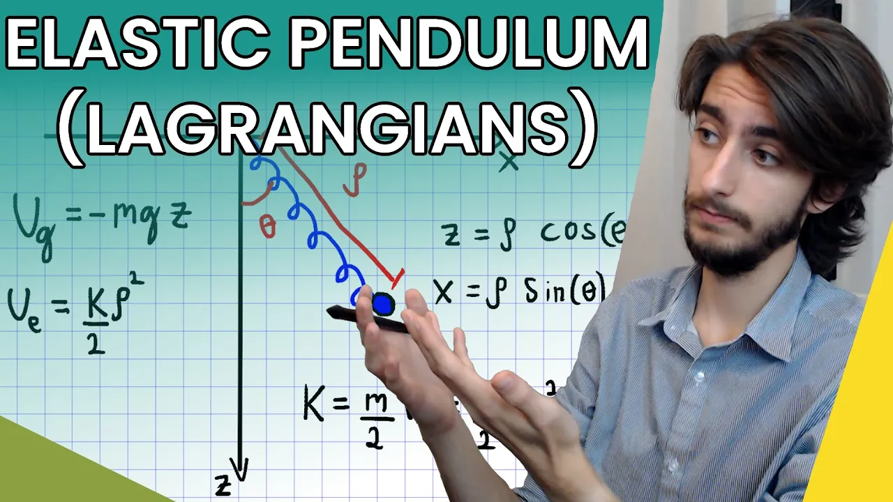
Lagrangian mechanics, which provides the analytical framework to derive the equations of motion for complex, constrained systems.
Chaos theory and the butterfly effect, studying how chaotic systems exhibit extreme sensitivity to initial conditions.
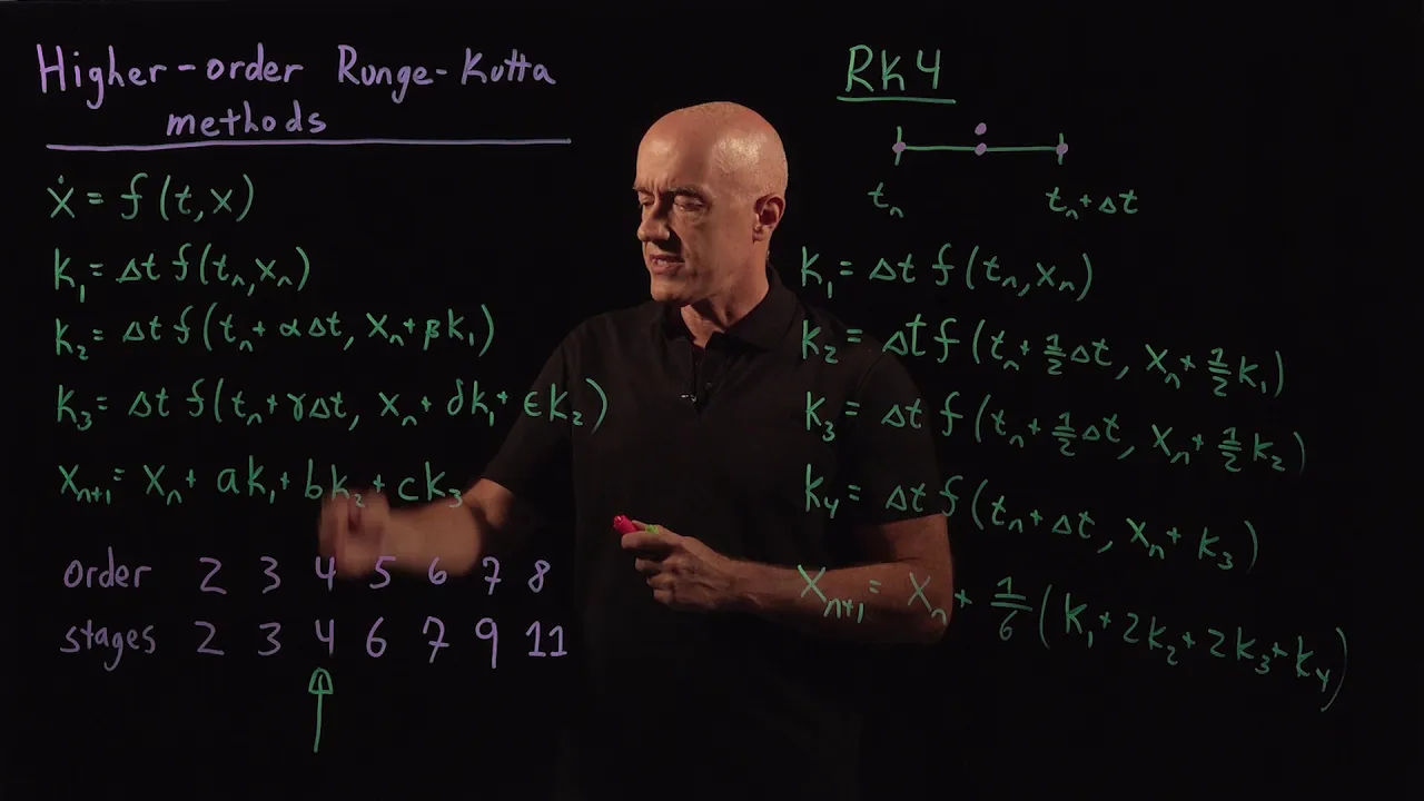
Advanced numerical solvers, such as the fourth-order Runge-Kutta (RK4) method, to prevent energy drift in the simulation.
Generalizing the simulation to N-pendulum systems or incorporating elastic connections (spring-pendulums).
929.5K views19Klikes31:11Original Release: 2018-02-13
hello and welcome to a coding challenge today I'm going to attempt to make a double pendulum simulation now I actually don't have a coding challenge that's a single pendulum so I should double back double back and make the single pendulum challenge I do have some videos about pendulum simulations in my nature of code playlist which I will refer you to but I really always want to make the double pendulum because it's like this crazy it's creates a double pendulum which if you figured out already is the having tube a pendulum attached to another pendulum as you swing the double pendulum and you trace the path of the bottom point it makes these beautiful chaotic kind of insane patterns and you can see an image of it here from some other YouTube video that you could probably go and find and watch so this has been on the coding challenge list since June 24th 2016 and this most recently I looked at it and back in December and I found this wonderful reference and so oh look at this oh this is is this the reference I wanted to look at yeah so we can actually just let's look at this here let's we're basically I want to make this so ok so this is what I want to make right there there's the double pendulum so but really what I need is the formulas on this page so let's first establish let's establish for ourselves this diagram so what I need for a double pendulum is this I'm going to consider to be point zero zero then this I'm going to consider to be point x1y1 and this here and let me let me be more thoughtful about how I draw these lines this here I'm going to consider a point x2y2 so there are important variables here well there's a bunch of things there's the year that in theory there are two what you might call Bob's the Bob being this thing at the end of a pendulum so there's the mass of this one which is mass one there's the mass of this one which is mass - okay I also need to keep track of this length arm length the arm of the pendulum so I'm gonna call this one r1 and r2 I now I just realized that if you look at the web page of looking and they called it l1 and l2 but I'm gonna call it r1 because variable name L and code it looks like a 1 it's very confusing so r1 and r2 then what's really important is I have two angles I have this angle here theta one and then now what's the best way for me I think so let me draw it I have to get let me I I want to be able to see that angle so let me draw it out like this so this being fada to now this is x2 y2 and this is r2 and this is m2 okay I think I've got this pretty much right these are all the variables of my system the only thing that I really need to keep track of is theta 1 and theta 2 R 1 and R 2 I'm going to be calculating where these points are based on those angles okay so this is this is the diagram so that means I'm gonna do this in processing that means I can start by having oh yeah I guess yeah I kind of that's this is I wouldn't might have been backwards about the theta 2 angle but I know it's fine it's fine it's fine I'm good I'm good let's see well we'll find out if we made a mistake later so I'm gonna say I need R 1 it's gonna be 100 oh I mean I mean I forgot I was in processing R 1 is 100 R 2 is also 100 let's just have a mass 1 be 10 I'm making these up mass to be 10 you know there's also so then I the lengths amass and any this this point 0 0 so I'm gonna need okay so then I need set up then I need draw and I'm going to create a window that is let's make it 600 by 600 and we'll say background 0 and then stroke let's make it back around 255 stroke zero let's make everything a little bit thicker so we can see it stroke wait - and now what do I need to do let's first Trant let's run this the first thing I want to do and if you want to move this over a little bit here the first thing that I want to do is I want the zero zero point to be like here in the middle so the way to do that so I'm just gonna use translate so I'm going to say translate to 300 comma 50 and then I'm gonna what I need to do is I've need to calculate X 1 and X 2 so X 1 equals we just need a little trigonometry right so how do I get to this point how do I get to this point well I need to know how what's my y offset and what's my X offset and you might realize now this is a little bit weird it's a little bit of a different scenario because X is actually across from the angle sine of that angle theta 1 equals x divided by R 1 so X actually equals R 1 times the sine of theta 1 okay so now I need to I can calculate X 1 equals R 1 times what did I say sine of oh I don't have the angle so let me create two variables a 1 is 0 a 2 angle 1 angle 2 sine of a 1 y 1 equals R 1 times cosine of a 1 it's a little backwards than what you might see in a lot of other polar to Cartesian videos and then I'm gonna say line from 0 0 x 1 y 1 and then I'll draw a nice little lips there x 1 y 1 16:16 and you know I have this mass so I probably should actually draw of it relative to the mass so let's draw it like just call it m1 and then let's make sure I say fill 0 let's run this there we go so we can see this is the top of the pendulum and let's make the let's make it a little bit longer and a little bit bigger okay so that's good that's the top of the pendulum that looks right now what I need to do is calculate x2 which is our two times sine of a - the same exact math is going to apply our two times cosine of a - but it's offset from x1 right y1 x1 y1 right because this is going to calculate it according to this angle in the same way but the offsets the y offset and the X offset are relative to x1 y1 so I could use translators rotate but I'm just gonna add the offset in there and now to render that I should be able to say line now I want the line to go - let's be let's be I'm gonna be like so it'll retentive about this I want to start with x1 y1 x2 y2 and then draw that next ellipse and we should see there we go so this is looking good now let's just see am I crazy is this right so like for example there's no animation happening yet but if I were to say something like you know pi divided by 2 that's 90 degrees yeah okay so that's right and if I were to say like pi divided by 8 and PI divided by 4 that makes sense right so the angle is the angle and the length is what's controlling where everything is positioned and I could start doing weird stuff like I could just say like for no reason like a1 plus equal zero point one and you can see it's doing that so I in some ways I have but this is not the actual formulas for the mechanics of how a double pendulum now interestingly enough this is an interesting sketch just on its own because now I can have that go the other way and we can see well you know what's going on here so one thing I want to add to this just while we're here let me add the tracing pross prop let me add the tracing of the path and I'm gonna do this in a kind of funny way I'm gonna create a P graphics object and I'm gonna call it I'm gonna call it I'm in about canvas I kind of don't want to call canvas because when I make the p5.js version of this I don't want it to be canvas but I'm gonna do that anyway so I'm gonna say canvas equals create graphics 600 600 and then I'm gonna say inside draw I'm gonna say canvas dot begin I'm gonna do this at the end what I want to do basically and then I'm gonna draw the background no canvas top begin draw so this is an off-screen graphics context the same as the thing that you are seeing in the window but the reason why I want to use it is because I want to draw the background on it only once so I can have nice trails and then what I'm gonna do is at the end here I probably should have waited this to later I don't know why I'm doing this now but it's the order that I'm doing it in I'm gonna draw just a point at what I need to translate canvas translate and you do that same translation 350 so 300 comma 50 and draw a point at X x2 y2 so I'll make it a line or something later I just want to see ok and now if at the beginning I actually draw that as the background image canvas 0 0 canvas dot stroke wait for canvas stroke 0 there we go so you can see this pattern that it's doing there's kind of like very similar to like to pull a road stuff because really what we have is just some oscillating going on but I want it to be an actual double pendulum so not just some arbitrary angle changing okay now so what's interesting what's going on here this is actually a 1 is changing by a value remember this I don't know if you remember this but if you've watched any of my other videos I've kind of got these physics engines in a lot of places the position changes by the velocity the velocity changes by the acceleration there's this concept of a derivative the change in overtime is the velocity the change in velocity over time is the acceleration or I can say a 1 so I could say something like a 1 velocity is point 1 right let me let me declare some more variables so I want an A 1 velocity to be 0 and I want an A 2 velocity to be 0 then I also want to have a 1 acceleration to and have those B 0 as well so there we'll see the notation on that on that page for a second so what this is what I want to do I really want to have a 1 change by a 1 velocity a to change by a 2 velocity and then I also want to have a 1 velocity change by a 1 acceleration a to velocity change by a 2 acceleration now not being very thoughtful about time I'm just thinking of one frame as one unit of time so I'm going to do one adjustment to the angle where as you know if I'm really trying to be more accurate about this I might try to do several iterations of the math per frame that would make more sense later as I get a little further here but this should give me the structure from which to to do this so if I run this now once again it's not moving but let's just give a little let's give it a little bit of acceleration 0.01 let's make this one negative 0.001 because there now it's accelerating out of control really fast because those numbers are accumulating on each other but you can see this is kind of the idea I need to figure out what are those acceleration values of the angles and if you go and watch my simple pendulum video you'll see it's kind of an easy thing to calculate based on gravity really simple formula the thing about the double pendulum is and I'm not going to derive these formulas but as I scroll through this page it's going to actually attempt to derive those formulas of motion I'm just going to scroll down and get to the end here we go this is what I'm looking for these two this is what looks like double quotes is prime prime so theta 1 prime is velocity the angular velocity theta 1 prime prime is the end the acceleration so all I need to do no problem I'm just gonna implement these formulas in my code and we'll be done actually when I just end this video right now you do that I'll be back here okay you're probably still here did you pause the video and do it yourself this is gonna be um so I'm gonna I'm let's see what's the best way for me to do this what I'm gonna do is whoops I'm in the wrong place is I'm gonna move this over here I need a little more space I'm gonna actually just take a screenshot of this absurdly because I want to be able to see it and look at my code at the same time so I should be able to go now to the I don't need this open should be able to go to the desktop where I have that screenshot and I've got that up there now and let's lower my processing window to down here okay so let's find a place where I can actually implement this so I'll just do it at the top of draw theta1 angular 1 a equals now i just need to put all of that stuff in my code so what 10 when I see like a formula like this it's kind of like I don't want to write this all in one line of code it's gonna be crazy I like to break it up into parts so first of all there's definitely two parts there's the numerator which is the top of that in the denominator but there's also kind of parts of the numerator because there's like this whole thing - this whole thing - this whole thing so let me start doing it that way let me say float numerator 1 equals negative G tonight do I have a variable called G so G is the universal gravitational constant I assumed that's just going to be 1 but we could play with that to change kind of like the strength of gravity there's a real-world number that that is but I don't care about for the purpose of this video so in a way I would have liked to take it out but I'm gonna leave it in there negative G times 2 what let's put parentheses 2 times m1 plus m2 times sine of angle 1 so that's one thing the next one is and please those of you live following along tell me if I make a mistake here the next one is negative m2 times G times sine of angle 1 minus 2 times angle then the third part here is negative 2 times sine angle 1 minus angle 2 times M - oh boy oh boy x okay hmm let's make this let's make the next thing M for which is oh and this so theta 2 prime is in my my notation is angle to underscore V I probably could have thought of a different name so it's the velocity times R 2 plus angle one underscore velocity o squared this is squared - oh my goodness so that's squared so angle two velocity times itself squared times R two plus angle one velocity times itself times R one times cosine of angle one minus angle two I think and there's be parentheses around this whole thing but since I made it its own thing I don't have to and then the denominator denominator is R one's gonna be little easier times two times M 1 plus M 2 minus M two times cosine of two times angle one minus 2 times angle 2 okay so now assuming I didn't make a mistake which I'm sure I did angle one acceleration equals numerator 1 plus numerator 2 plus numerator 3 times times numerator 4 I think that's correct that's all the divided by denominator and parentheses around all of this oh ok I I almost want to just just do that like let's just run it with this and just say that angle to acceleration is 0 and by the way this could be a local variable there's no reason to have this be a global variable because gonna get recalculated every frame so let's take these out here and let's just see like syntax wise does this even run oh boy float angle one oh I forgot to semicolon okay so this is promising why because that looks like a single pendulum now it's kind of spitting a little bit out of control so like probably going to want to add some dampening but this is right it's going in a perfect circle so I'm not totally insane I've got something that's working here that's kind of nice okay now time for formula number two and by the way somebody in the chat asked what crazy person thought up this formula nobody crazy thought it up somebody crazy calculated it probably not so crazy somebody who's really very thoughtful and kind and really likes pendulums and another video I'm sure could go through the math of this but I like sometimes I like it when I'm like oh the coding train is not about deriving the math just implementing it so today is a day for that so now I need to do well it's not going to let me read eclair these variables so let's do let's do let's just use them again whatever let's say two times sine of angle 1 minus minus angle 2 times do I dare like keep going here I'm going to Derek keep going no no let's do the numerator 2 equals angle 1 velocity squared times R times m1 plus m2 okay that's 1 R 1 that's R 1 so easy to make a mistake here numerator 3 equals G times m1 plus m2 times cosine of angle 1 ok numerator 4 equals angle 1 where am I looking no angle 2 V squared times R to 2 times m2 times cosine of angle 1 minus angle 2 and if I look here at this these are the same right the denominators are the same the only thing that's different is l1 and l2 double check double check double check yes so I could copy paste this code here and bring it down here and just say r2 now this now equals write its numerator 1 times numerator 2 plus numerator 3 plus plus numerator 4 divided by denominator oh my god what is the chance that this is actually correct what is the chance that this is correct very very oh oh oh I'm being told that I have some transcription errors make it denominator 2 I did that and a 2 a equals num1 x okay hold on hold on let's look at a 2 a num 1 x num2 now i'm one time zone 2 + num 3 plus number 4 I think that's fine I think I'm good oh there's a squiggly line here yeah num for is num 4 is 8 2 squared times R 2 times M 2 times cosine of a 1 I think I'm good I think I'm good 34 I need a parentheses I think I'm good I'm gonna run it does that look right no okay something's wrong something is definitely wrong ok let's look at the let's let's look at the denominator L 2 times 2 times M 1 plus M 2 minus two times cosine of two times angle 1 minus 2 times angle - that looks correct ah okay I'm seeing in the chat this I think I need to be more thoughtful oh there's a parenthesis oh this parenthesis goes all the way to there oh that's very wrong very very wrong thank you so this is this times all of that added together so this parenthesis needs to be here there we go I think now no no not in denominator numerator 4 that's why okay okay this numerator 4 no no no no no no not a numerator 4 I was doing so well it's in the end this parenthesis cause here there we go right because when I put this all together I need this thing times these 3 things added together with parenthesis around it and if I want to be really safe about this I'll put another parenthesis around it okay okay now okay okay all right that looks kind of like a double pendulum whoa now it's got quite a bounce to it I don't know I've actually done it right it is kind of spiraling out of control which I think maybe my I might have an issue that so let's think about what could be the problem here I don't think the order matters I've because putting it here is the same as you know just not doing it the first frame oh yeah well yes it would be I should put this is correct that this makes more sense to put here yeah I think I actually have this correct I think the issue is some oh that really just weird did that did I do something that fixed it oh yeah interesting oh that does matter I was thinking that this doesn't really matter but I I mean I definitely the the correct way to do it would be to adjust the velocity first based on the force which is the acceleration and then adjust the position somehow that seemed to have fixed it there's also some yeah so okay so let's actually get it to do so couple things one is I won a half I want to have previous x2 and previous x1 and what I want to do is I want to actually draw a line I want to trace the line from ech previous X to previous Y - is that what I put here previous x2 previous Y to you and I'm gonna have these be can I say that no can't have a float so just like set them equal to negative 1 or something and so here what I want to do as soon as I as soon as I calculate this I want to save I would have to do it afterwards I want to say at the end I want to save the previous previous why to and I only want to draw the line if previous X 2 is not equal to negative 1 I said a better way to like not draw that first line actually I could just say if frame count is greater than 1 okay I just wanted to do that so I could least draw the full pack so let's actually have it start let's let's do a couple things remember one is let's have it start let's have a variable called Center X and Center Y and as soon as I set the size let's say Center x equals with divided by 2 and Center y equals 50 that way I can reuse those Center ex-senator why because I need that also here Center X Center why I want to be able to see a bit more of the canvas so I'm gonna say like 900 oops Oh and why why is my background up with this needs to be the same size with height okay it's a little bit better now now let's actually have it start higher up let's have it start pi divided by 2 pi divided by 2 let's see what happens here so this should be its and I missed I think this is the right pattern I don't know what initial settings to give it but it kind of looks like looks pretty simple similar to what I started with when I did that google image search right if you remember my Google image search at the beginning of this video this one out looks pretty similar to that so I think I have now done the double pendulum now how I know this thing is playing with the mass playing with the G value playing with the different are values playing with the color there is so much that you could do with this and you know I could also one thing that I think might be worth just noting here and I absolutely would like to also have this I think I want to have a much lighter trace right so I have this one thing a couple things that might be worth noting here is that what was I gonna say oh yeah I could add some dampening so one thing I could do is say like I could simulate this idea of like friction or air resistance by saying a 1 that x equals 0.99 9 so it's always losing a little angular velocity every frame so we could do this so this should I mean it might take a very long time but this should eventually dampen those values so that it comes to arrest so that's something they sort of play with I mean certainly if I just to show that effect really strongly if I put like 0.9 if it's losing 10% of its you can see that it's it's like it's almost as if it's like swinging through mud so that's one thing that we can kind of play with a kid stuff and when I when you make when this gets poured into p5.js as a JavaScript version could have sliders to play with all this stuff but you can see what that really does the dampening really causes it to not be able to swing so I'm gonna comment this out though and leave this in the code the other thing that I would do is you know what does it mean if the mass of these is 20 you know how does that affect the pattern that I'm gonna get what if I make the art the arm length of the first one like 50 right and the second one like 400 you know this is sort of interesting what do I get what kind of pattern do I get here so there's so many possibilities so this come this is the end of this coding challenge the double pendulum coma challenge this I think is one which is really ripe for your variations up for your own take do your own twist on this how are you drawing it how are you visualizing it how you adding user interface controls is that the kind of thing that you make how do you make it interactive there's so many possibilities here how are you drawing the trail oh I got to stop so I hope you enjoyed this coding challenge I would not be super more gravity being told I could also change the force of gravity let me put this back up to something more reasonable right if I make gravity really strong you can see what kind of like craziness happens versus gravity really weak you can see an almost just more likely only kamancheh this double pendulum on the moon so to speak 3d version would be crazy I can't make a 3d version so I would love for you to make your variations of this it says share them with me the coding train comm actually now has a system a way for it's not the most obvious thing but it's tied to a github repository where you can submit a pull request go check that out there'll be a link in this video's description for how to do that and I will also have a JavaScript version of this that runs in the browser which the code will essentially look exactly the same so thanks for watching and I will see you wha in a future coding challenge you
Up Next
12:51
Chaos Theory and the Butterfly Effect: Determinism vs. Predictability
@veritasium
7.7M views•2019-12-06

12:53
21cm Hyperfine Transition in Neutral Hydrogen: Radio Astronomy Basics
@AaronRobertParsons
12.4K views•2011-10-13

32:32
NMR Spin Physics I: Zeeman Effect, Resonance Condition & Larmor Frequency
@nptel-indianinstituteofsci8064
2.3K views•2024-01-17

27:14
Entropy and the Second Law of Thermodynamics Explained
@veritasium
27.5M views•2023-07-01
Related Study Plans & Knowledge Roadmaps
Structured learning paths in Physics
physics
Nuclear Physics (Decay, Fission & Reactors)
01Atomic Structure and the Binding Force
02Radioactive Decay and Half-Life
03Nuclear Fission Mechanics and Chain Reactions
+ 2 more learning modules
12h5 modules
Explore Roadmap
physics
Soft Matter (Polymers, Colloids & Rheology)
01Foundations of Soft Matter & Thermal Forces
02Polymer Physics and Macromolecules
03Colloids, Surfactants, and Self-Assembly
+ 2 more learning modules
38h5 modules
Explore Roadmap
physics
Analytical Mechanics: Lagrangian & Hamiltonian
01Mathematical Foundations: Calculus of Variations
02From Newtonian Mechanics to Constraint Dynamics
03The Principle of Least Action & Lagrangian Mechanics
+ 3 more learning modules
28h6 modules
Explore Roadmap
physics
General Relativity (Spacetime & Cosmology)
01Foundations of Relativity: Special Relativity
02The Geometry of Spacetime: Equivalence Principle & Curvature
03Einstein's Field Equations: The Mathematics of Gravity
+ 2 more learning modules
55h5 modules
Explore Roadmap