













![[다변수 미적분 심화 스터디] Connection에서 Riemannian curvature tensor로](https://i.ytimg.com/vi/snNrsEnaURA/maxresdefault.jpg)


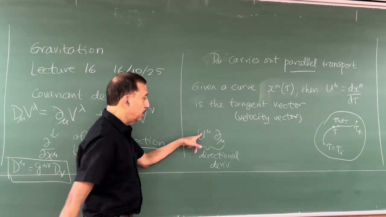


Christoffel symbols are mathematical quantities that describe how basis vectors change as they are transported along different coordinate directions in a curved space, calculated using the Levi-Civita connection which ensures that changes in one direction are compensated by changes in another; in polar coordinates, these symbols reveal that while radial basis vectors remain unchanged, angular basis vectors rotate by an angle equal to the radial coordinate when transported radially, and gain radial components proportional to 1/r when transported angularly, enabling the reconstruction of true Cartesian geometry from the distorted polar coordinate system.
Conceptualizing Christoffel Symbols in Curvilinear Coordinates
Added:Familiarity with curvilinear coordinate systems (such as polar, cylindrical, and spherical coordinates) and how basis vectors change positionally.
Basic understanding of the metric tensor and how it defines distances and inner products in different coordinate spaces.
A strong foundation in multivariable calculus, particularly partial differentiation, coordinate transformations, and the chain rule.
An introductory understanding of tensor notation, index notation, and the Einstein summation convention.
Formulating and solving the Geodesic Equation to determine the shortest or straightest paths in curved spaces.
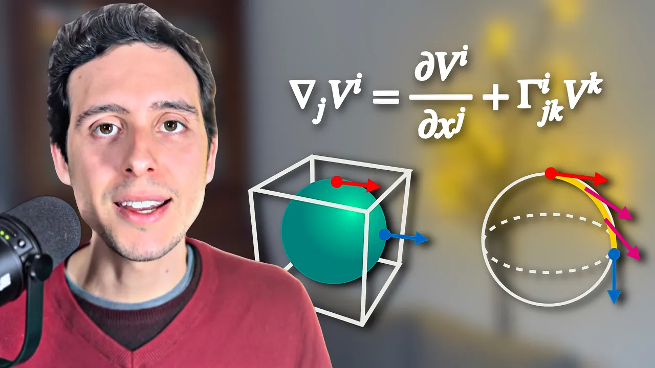
Mastering the Covariant Derivative, which generalizes the derivative of vector fields to curved manifolds using Christoffel symbols.
Defining and calculating the Riemann Curvature Tensor to measure the intrinsic curvature of a manifold.
Applying these mathematical structures to General Relativity to understand how matter and energy curve spacetime.
201.4K views9Klikes23:38Original Release: 2023-10-07
If you've traveled on an airplane before you might have noticed that the shortest route to your destination doesn't take you along a straight line on the map but rather follows a curved path. This is an example of what's called a geodesic, a route representing the straightest path on a surface, and to calculate it you need the aid of certain mathematical tools known as the Christoffel Symbols. Likewise in general relativity these same tools allow you to calculate the inertial routes of objects through space and time. But where do such tools come from and how can we understand them intuitively? This is Dialect with Conceptualizing the Christoffel Symbols. This is Cartesian bear, he lives in Cartesian land, where lines are all straights and intersect at right angles this is polar bear he lives in polar land where lines are all straight and intersect at right angles. Okay aren't these two lands exactly the same thing? Well sure, but not quite. You see Cartesian Bear lives in the real world, where his grid distances and coordinate angles match up to actual distances and actual angles, while Polar Bear is living in a matrix, a false projective world like the map on your airplane screen. What this means is that when Polar Bear moves in a straight line along his Theta coordinate direction in polar land, he actually moves along a circle in the real world. And when Polar Bear moves in a straight line in the r coordinate direction in polar land he actually moves radially outwards in the real world, as if along the spokes of a wheel. Polar Bear is unaware of all this because he assumed his coordinates to represent independent dimensions and so to him Polar Land is perfectly Cartesian. But one day Cartesian Bear decides to Red Pill poor Polar Bear. "Your idea of reality is actually a map," he tells Polar Bear, a projection due to the false way you constructed your coordinates. Now Polar Bear descends into an existential crisis. How can he know what's real and what's not? Before in order to measure distances and angles in Polar Land he had always relied on his basis vectors ER and E Theta. Across Polar Land these basis vectors always had unit length one and everywhere were oriented at right angles to one another. But since realizing he lives in The Matrix, Polar Bear now knows that the lengths of these basis vectors don't represent true real world lengths, nor does the right angle between them necessarily represent a real right angle.
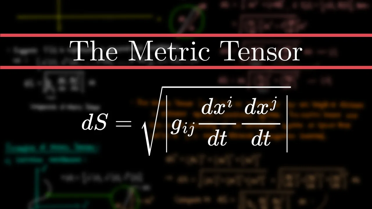
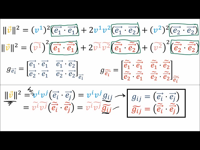
Moreover, the amounts of distance and the angle these basis vectors do represent could actually change from point to point across Polar Land. Fortunately for Polar Bear we will provide him with a useful mathematical tool known as the Metric Tensor. If Polar Land is a map of sorts then this tool is like a bar scale for his basis vectors. It tells him at every point across Polar Land how much real world distance his basis vectors represent and what the real world angle between them is. In this case the first component of the metric tensor is one, so this tells polar bear that everywhere in polar land his ER basis vector correctly represents one unit of real world length. Thus if polar bear moves one unit of R coordinate distance in Polar Land, he knows he'll also have moved one unit of distance in the real world. The second component r-squared tells Polar Bear that his Theta basis vector represents as many units of real world distance as is equal to whatever R coordinate he is located at. So if Polar Bear is located at R coordinate 2 and moves one unit of theta coordinate distance, he will move two units of distance in the real world. And if he's located at R coordinate 4 and moves one unit of theta coordinate distance, he will move four units of distance in the real world. This should make intuitive sense for polar coordinates because any change in angle will sweep out a greater distance farther out from the origin. Finally the last two components of the metric tensor are both zero, which tell polar bear that the 90° angle between his basis vectors represents 90 degrees in the real world as well. So it turns out that Polar Bear's theta ruler essentially grows in length as he moves radially outwards in the real world. This explains in part why his coordinate construction of Polar Land was false to begin with; however there is more to the story, for as Cartesian bear can plainly see, when Polar bear moves along a circle the direction in which he lays out his rulers also steadily rotates and changes. Polar Bear is still unaware of this however, because although the metric tensor tells him about the real world lengths of his basis vectors and the relative angle between them it doesn't explicitly specify anything about the real world orientation of those vectors. But is it still possible for Polar Bear to deduce such information from the metric tensor alone? Let's have Polar Bear consider just four infinitesimal pieces of Polar Land at a certain R distance out from the coordinate origin. Each piece has length DR and height D-Theta. We'll help him out by drawing the ER and E-Theta basis vectors on each piece. Now keep in mind that the basis vectors have a unit length of one, even though we are drawing them as being on par with the infinitesimal lengths of our pieces. Now the r coordinates of the pieces in the first column we'll label as R and the r coordinates of the pieces in the second column as r + DR. Similarly the theta coordinates of the rows we'll label as theta and theta plus d- theta. Now let's resize these pieces to match their real world areas using the metric tensor.
We start by multiply in R lengths everywhere by one. Obviously this means the DR lengths of all the pieces as well as the lengths of all the R bases vectors remain the same. Next, we multiply D-Theta lengths everywhere by their R coordinate distance out from the origin. This means the D Theta lengths of the pieces in the first column become r d Theta while the Theta bases vectors are resized to length R. In this the second column meanwhile the D Theta lengths of the pieces become r + Dr * D-Theta and the theta basis vector lengths become R plus Dr. Polar Bear now has four properly sized pieces of Cartesian Land, and so to figure out the real world orientation of his basis vectors, all he needs to do is fit these pieces together like a puzzle. Indeed, should he find a general method for fitting pieces together at any arbitrary coordinate, then this would allow him to fit together every resized piece of Polar Land, so as to reconstruct the whole of Cartesian Land and be able to determine his geodesics upon it. But how does he go about this using just the information of the metric tensor alone? Well let's examine each metric component more deeply to see what it's saying. Now the fact that the first component tells us that our lengths everywhere are unchanging means there is no one-dimensional curvature in the R direction in Polar Land. In terms of our resized pieces this means we can thus conjoin our two columns side by side without bending or rotating them.
Meanwhile the fact that the second component tells us that the theta lengths do change across Polar Land means we won't be able to preserve the straightness of the theta direction, and thus that our rows will have to be bent into another dimension to be connected. Lastly if we consider the second partial derivative of the Theta component we see that it's a constant which hints to us that we need only one extra dimension in order to accommodate this bending or curving, and so won't have to worry about bringing a third dimension into the picture. Now from visual intuition alone you've probably already guessed that we need to bend the rows so that they're touching like this, and if you're familiar with polar coordinates you could reasonably surmise that the angle through which they should be rotated is D-Theta. But how do we extract this information from the metric tensor? Well to do that we need to invoke something called the Levi-Civita connection. For infinitesimals like this, this connection is expressed as a simple equality stating that the change in our e-theta basis vector when transported along the radial direction must equal the change of our ER basis vector when transported in the theta direction. What does this equality mean visually? Well consider these two square infinitesimal pieces of Polar Land side by side. If we transform the theta lengths of one of the pieces while keeping the other constant we've now added extra physical space to our manifold. This amount of new length is tracked by noting the change in the E-Theta basis vector. Now to keep the manifold continuous there needs to be a change in the radial basis vector of the next piece atop the first which will compensate for this new length. Obviously the radial basis vector just simply growing or shrinking won't compensate for this extra length since it lies in a wholly different dimension.
Thus the radial basis vector must be rotated in order to supply the additional length. Now if the theta growth is small, then this rotation will likewise be small.
But if the theta growth is large, then so too will the required rotation be large. So how quickly theta lengths are growing along the radial direction will in fact determine how rapidly Polar Bear's basis vectors are rotating when transported along the theta direction. Indeed it is this Levi-Civita condition that the growing or shrinking of Polar Land along one dimension be compensated by its curving into another dimension that ultimately causes the rotation of Polar Bear's coordinates in the real world. But what is the amount of this rotation precisely? Well returning to our infinitesimal pieces recall that this lower left piece has a resized theta length R D-Theta while the lower right piece has a resized Theta length R plus R D-Theta. The difference in theta lengths between the lower left and lower right pieces is thus R + DR D-Theta minus R D-Theta which equals DR * d-Theta.
Now the length produced when a radial segment R is rotated through a small angle D-Theta is R * D-Theta. Here the length of our radial segment is DR which means to produce the length DR D-Theta it needs to be rotated through an angle D-Theta.
Polar Bear is feeling better about his reality; the metric tensor gave him the real world lengths of his basis vectors and the real world value of their adjoining angle, and now the Levi-Civita connection gave him the real world orientation of these basis vectors. Indeed, armed with such knowledge he now possesses all the requisite information for how to properly connect his resized infinitesimal pieces of Polar Land. He simply conjoins the columns in the radial direction side-by-side and then tilts the top row through an angle D-Theta and voila, he is looking no longer at the false geometry of Polar Land but rather at the true geometry of Cartesian Land.
Now it's time for him to formalize this process by describing precisely how the real world vectors corresponding to his Polar Land basis vectors will change as they are transported along different coordinate directions.
Since he has two basis vectors and there are two coordinate directions in which these vectors can be transported he will require four derivative vectors to fully describe such change. Each of these derivative vectors will in turn have two components, meaning eight total numbers will become involved and it is these eight numbers which are known as the Christoffel symbols. The Christoffel symbols are notated with three indices: the upper index indicates which component of the derivative vector is being referred to, the lower left index indicates which basis vector is having its derivative taken, and the lower right index indicates in which coordinate direction we are taking that derivative.
All right, now let's figure out what these symbols are by calculating each derivative vector. We'll start with the easy one: we'll take the R-basis vector and transport it a coordinate distance DR in the R direction in Polar Land. Here there is no change in this basis vector in the real world whatsoever, so its derivative vector is zero, meaning our first two Christoffel symbols are likewise both zero. Next let's take the theta basis vector and transport it along a coordinate distance D-Theta in the theta direction in Polar Land. When we do this, the real world Cartesian vector is rotated counterclockwise through an angle D-Theta. The change in this vector equals the length produced by this rotation and since the real-world vector had a length R the length produced by its rotation should equal R D-Theta. Now in this infinitesimal picture it's easy to see that this rotation occurs relative to the prior piece, but let's take a moment to look at the continuous picture in Cartesian Land. Here we have the transformed Theta Vector scaled to its proper length, and as we transport it through a small angle D-Theta the vector rotates accordingly. But what do we measure its rotation relative to? Well in this case, we'll transport a second vector alongside it which maintains a constant orientation in the direction in which the theta vector was initially pointing before it was transported. Then we can see that the change in the theta vector is a change relative to this second vector. This is essentially the same thing we did in the infinitesimal case but in the continuous case it's referred to as parallel transport.
Returning to our calculations, Polar Bear's theta basis vector thus changes by an amount R D-Theta in the real world per coordinate distance D-Theta in Polar Land, so the relevant derivative here is R D-Theta / D-Theta which equals simply R.
The direction this derivative vector is pointing meanwhile is in the negative radial direction.
Now at different points across Cartesian Land such a vector will look like this; while at different points across Polar Land it will look like this. If we were to express this vector in its Cartesian basis we would get the components minus r cosine of theta in the X hat direction and minus r sine of theta in the Y hat direction. In Polar Land however we see that the components of this vector are minus r in the r hat direction and zero in the theta hat direction. Our next two Christoffel components are therefore minus r and zero.
Next, let's take the radial basis vector and transport it a coordinate distance D-Theta in the theta direction in Polar Land. In Cartesian Land this vector is again subjected to a rotation D-Theta and since its length is one, this rotation produces a length of simply D-Theta. D-Theta / D-Theta is 1 so the derivative vector everywhere in Cartesian Land has length one and points in the Theta coordinate direction.
However these vectors do not have length one like this everywhere in Polar Land, because if Polar Bear is expressing them in terms of his basis vectors, we must remember that his theta ruler length is growing across Cartesian Land.
At a certain R distance out in polar land Polar Bear's theta basis vector represents r Cartesian basis vectors, so if the derivative vector has the length of one Cartesian basis vector it must be shrunk in Polar Land to a distance of 1 / r. The components of the derivative vector are therefore zero in the r-hat direction and 1 divided by r in the theta-hat direction. These are our next two Christoffel symbols.
Last but not least, let's take our theta basis vector and transport it a length DR in the radial direction in Polar Land. In Cartesian Land the vector changes by length DR so its derivative is a vector with length DR / DR or 1 which points in the theta direction. Again normalizing this theta distance in Polar Land we see that our final two Christoffel components are again 0 and 1 / R. Now of course we could have short-cutted this process by remembering the Levi-Civita connection requires that that the derivative of the theta basis vector when transported in the r direction equal the derivative of the radial basis vector when transported in the theta direction.
With all eight Christoffel symbols calculated Polar Bear now has a much stronger grasp on reality. These symbols will tell him precisely the rate at which his real-world basis vectors are changing with respect to changes in his coordinate system. So for instance if he traverses an infinitesimal length D-Theta in Polar Land he knows his real world theta basis vector will shift to the left due to picking up a radial component equal to the Christoffel component there time D-Theta.
If he wants to counter this shift and continue traveling as straight as possible in the real world he will need to veer rightwards in Polar Land by an amount which will compensate for this component, in this case R D-Theta.
Indeed from this knowledge he can begin constructing something which will prove extremely important to him -- his geodesic paths across Polar Land.
Yes, it's a happy ending for Polar Bear who has finally made his way to the real world. But for us, we have only begun to scratch the surface of the Christoffel symbols. In ensuing installments we will need to make the relationship between basis vectors, the Christoffel symbols and the metric tensor explicitly precise; we will need to begin training for the index olympics; we will need to move from flat surfaces to curved ones; and lastly we will need to understand how to swap physical manifolds for spacetime manifolds. But to really truly understand relativity, there is only one revelation you need to make. You are Polar Bear -- you are the one living in The Matrix. This has been Dialect, thanks for watching.
Up Next
29:13
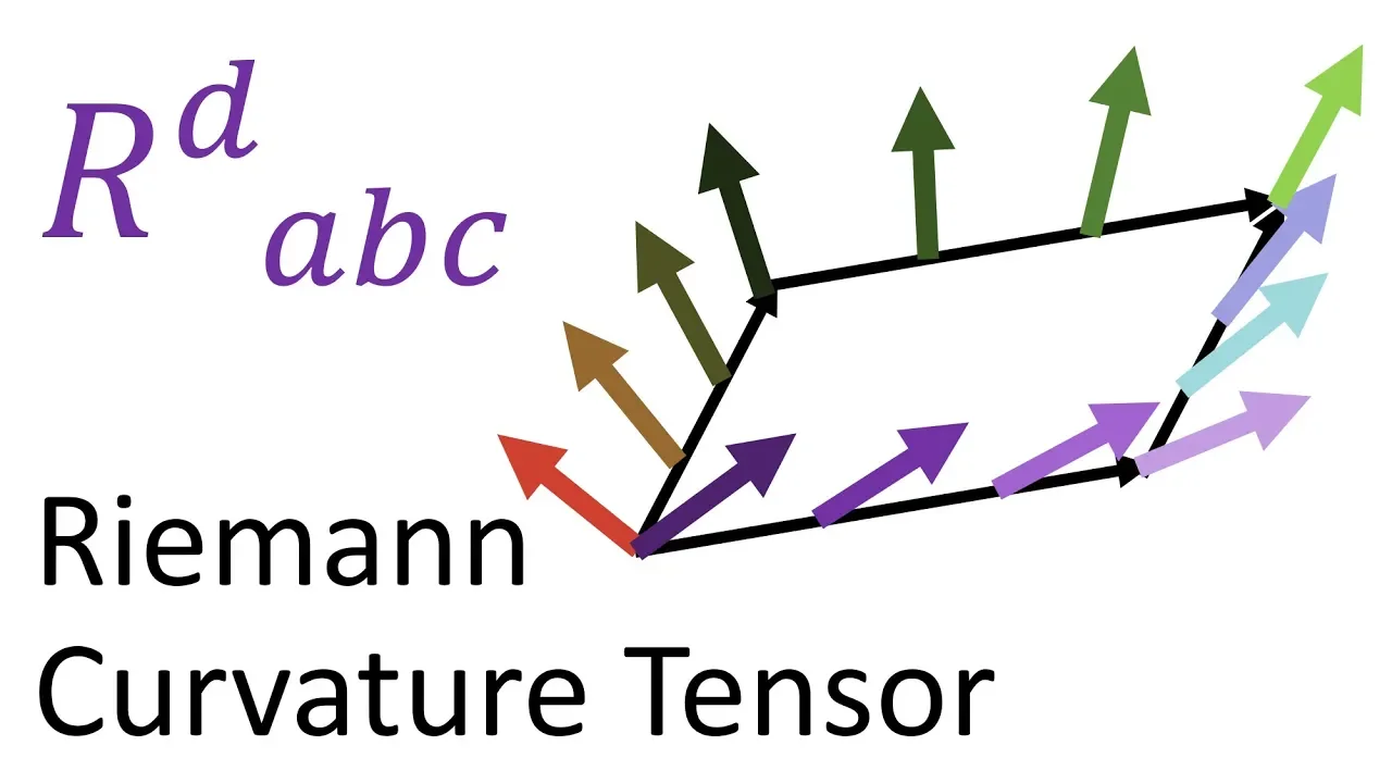
Riemann Curvature Tensor: Geometric Meaning in Tensor Calculus
@eigenchris
131.7K views•2019-06-16

4:43
Elliptic Curve Cryptography Explained: ECC, ECDSA, ECDH
@PracticalNetworking
28.5K views•2024-10-21

10:44
Fourier Series Introduction: The Big Idea Explained
@DrTrefor
387K views•2021-05-03

6:00
The Mathematical Impossibility of Accurate World Maps
@Vox
23.3M views•2016-12-02
Related Study Plans & Knowledge Roadmaps
Structured learning paths in Mathematics
mathematics
Tensor Calculus: Vectors to Riemann Curvature
01Mathematical Foundations: Linear Algebra & Calculus
02Covectors, Dual Spaces, and Tensor Basics
03The Metric Tensor and Index Gymnastics
+ 2 more learning modules
40h5 modules
Explore Roadmap
mathematics
Gödel's Incompleteness: Logic, Proofs & Limits
01Introduction to Formal Systems & Hilbert's Dream
02Set Theory, Cardinality, and Cantor's Diagonal Argument
03Arithmetization and Gödel Numbering
+ 2 more learning modules
14h5 modules
Explore Roadmap
mathematics
Galois Theory: Fields, Groups & Solvability
01Foundations of Abstract Algebra: Groups & Fields
02Polynomials & Field Extensions
03Splitting Fields & Symmetries
+ 2 more learning modules
24h5 modules
Explore Roadmap
mathematics
Non-Euclidean Geometry: Models & Geodesics
01Euclid's Fifth Postulate and the Birth of New Geometries
02Hyperbolic Space and the Poincaré Disk Model
03Geodesics: Defining Straight Lines in Curved Spaces
+ 2 more learning modules
15h5 modules
Explore Roadmap