Machine learning is a technology that enables computers to learn from data and make predictions or decisions without being explicitly programmed, with applications ranging from facial recognition in social media apps to recommendation systems and medical diagnosis tools.
Machine Learning with Python: A Beginner's Guide to AI Models
Added:Deep Dive
Basic Python programming syntax, including control flow, functions, and standard data structures like lists and dictionaries.

เรียนรู้พื้นฐานภาษา Python | High-level, Interpreted, General-purpose Programming language 👨💻💯
47.6K
Python has four main data structures for storing collections of data. Lists are ordered, mutable collections in square brackets, supporting mixed types and duplicates. Tuples are ordered, immutable collections in parentheses, useful for fixed data. Sets are unordered, mutable collections in curly braces, automatically removing duplicates. Dictionaries are unordered key-value pairs in curly braces, with unique keys and any value types. Each structure serves different purposes: lists for ordered collections, tuples for fixed data, sets for unique items, and dictionaries for key-based lookups. Control structures enable decision-making and repetition. If statements use indentation to define code blocks, with else and elif for multiple conditions. While loops repeat code while conditions are true, with break to exit early and continue to skip iterations. For loops iterate over sequences using the for variable in iterable syntax. Nested loops allow processing multi-dimensional data. Functions in Python are reusable code blocks defined with the def keyword, accepting parameters and returning values. Default parameter values allow flexible function calls. Lambda functions are anonymous functions defined with the lambda keyword, accepting any number of arguments but containing only one expression. They are useful for short operations, especially as arguments to higher-order functions like sorted() and filter().
Click to watch →
🐍 Python Basics & Syntax for Beginners | Learn Python Fundamentals Step by Step
1.6K
This section covers data structures, control flow, and functions. Strings are sequences of characters in quotes, supporting indexing (0-based), slicing (start:end), and looping. Methods include lower()/upper() for case changes, strip() for removing spaces, replace() for substitutions, split()/join() for breaking/combining, startswith()/endswith() for checking, isalpha()/isdigit() for validation, and find() for locating substrings. Lists are ordered, mutable collections in square brackets. Indexing accesses items by position. Slicing extracts portions. Adding uses append() (end), insert() (specific index), extend() (multiple items). Changing items uses list[index] = value. Removing uses remove() (by value), pop() (by index), del (by index/slice), clear() (empty all). Looping uses for item in list, range(len(list)), or enumerate(). Sets are unordered collections of unique items in curly braces, supporting add(), remove(), union, intersection, difference, and symmetric difference. Dictionaries are ordered key-value pairs in curly braces, accessed via dict[key] or dict.get(key), with add/update via dict[key] = value, removal via pop()/del/clear(), and looping via keys()/values()/items(). Control flow includes while loops (repeat while condition true) and for loops (repeat for each item in sequence). Range(start, stop) generates numbers. Break stops loops early; continue skips to next iteration. Functions are reusable code blocks defined with def, taking parameters and returning values. Print displays output; return sends values for storage and further use.
Click to watch →

كورس مابعد مقدمة الأساسيات في البرمجة
87.8K
Collections organize related data under single names. Lists store ordered data using square brackets with comma-separated elements. Dictionaries store key-value pairs using curly braces with colons. Access elements using indices (starting from 0) for lists or keys for dictionaries. Loops repeat code blocks: For loops iterate over collection elements, While loops repeat while conditions are true. Both require data, operations, and termination conditions. Infinite loops occur when termination conditions are never met. Python lists can contain mixed data types unlike some languages requiring uniform types.
Click to watch →

Python para principiantes | Python 101
1.8K
This section covers Python's core data structures and control flow mechanisms. Lists store multiple elements in a single variable using square brackets, supporting mixed data types, defined order, and duplicate elements. List indices start at 0, and methods like append(), insert(), and remove() modify lists. Dictionaries store key-value pairs using curly braces, enabling instant access through unique keys. Each dictionary element has an irrepetible key, and elements can be any data type including other dictionaries. Replacing elements uses the same syntax as adding new elements: dictionary[key] = new_value. Python executes code sequentially, but conditional statements allow selective execution. The 'if' statement executes its block only if the expression evaluates to True, requiring a colon and proper indentation. Six relational operators are covered: >, <, >=, <=, ==, and !=. The 'elif' statement provides additional conditional branches after 'if', creating cascading structures. The 'else' statement executes only if all previous conditions return False, and must be at the end of the structure.
Click to watch →
Python Tutorial for Beginners | Python Full Course From Scratch | Python Programming | Intellipaat
38.6K
Python has immutable (numbers, strings, tuples) and mutable (lists, dictionaries, sets) data types. Numbers include int, float, and complex types with automatic type detection. Strings support indexing, slicing, find(), replace(), split(), count(), upper(), max(), and min(). Tuples are immutable sequences supporting concatenation, repetition, indexing, and slicing. Lists are mutable sequences supporting append(), extend(), insert(), and remove(). Dictionaries are key-value pairs supporting access by key, len(), keys(), and values(). Sets are unordered unique collections supporting union(), intersection(), and difference(). Flow control statements control program execution: (1) if-else executes one block if condition is true, another if false. (2) Nested if-else checks multiple conditions sequentially. (3) for loop iterates over sequences (for x in sequence: statement). (4) while loop executes as long as condition is true. (5) break exits the loop immediately. (6) continue skips the current iteration and proceeds to the next. These statements enable decision-making and repetition in programs.
Click to watch →
Deep Dive
Familiarity with data manipulation and analysis libraries in Python, specifically Pandas and NumPy.
![[TUTORIAL] PYTHON para Análise de Dados - Aprenda do ZERO](https://i.ytimg.com/vi/FZODEbfcDwU/maxresdefault.jpg)
[TUTORIAL] PYTHON para Análise de Dados - Aprenda do ZERO
6.5K
This section introduces NumPy and pandas, the two most important libraries for data analysis in Python. NumPy is fundamental for numerical computations and serves as the foundation for pandas. To use NumPy, import it as 'np' and create arrays using np.array([values]). Arrays support element-wise mathematical operations like multiplication and addition. For statistical calculations, use np.mean(), np.sum(), np.min(), and np.max(). pandas is built on top of NumPy and provides DataFrames (two-dimensional tables) for data manipulation. Import pandas as 'pd' and load data using pd.read_csv('filename.csv'). View data with df.head() (first rows) and df.tail() (last rows). Get detailed information with df.info() and descriptive statistics with df.describe().
Click to watch →

A Gentle Introduction to Pandas Data Analysis (on Kaggle)
161.3K
To use pandas in Python, you must first import it using the statement 'import pandas as pd'. It is also common practice to import numpy as 'np' since pandas is built on top of numpy. These imports are essential for any pandas workflow.
Click to watch →

DSP | Special Lecture | SY DIPLOMA | K - Scheme 💻🚀
2.5K
Three standard Python packages for data science: 1) NumPy (Numerical Python) - provides support for large, multi-dimensional arrays and matrices, along with mathematical functions to operate on them efficiently. Used for numerical computations. 2) Pandas - a data manipulation and analysis library built on top of NumPy. It provides two main data structures: DataFrame (two-dimensional, like tables) and Series (one-dimensional). Used for data manipulation and analysis. 3) Matplotlib - a visualization library for creating charts, plots, and graphs. Used for visualizing data.
Click to watch →

КАК ИЗУЧАТЬ PYTHON / Lead Software Engineer Юрий Зайцев / АйТиБорода Shorts #3
56.7K
NumPy is a fundamental Python library for numerical computing and matrix operations. It provides efficient array handling and mathematical operations. Pandas is built on top of NumPy and provides higher-level abstractions for data manipulation through DataFrames. Both libraries are essential for data analysis and scientific computing in Python. They can be extended with C or C++ code for performance-critical operations while maintaining Python's convenient interface.
Click to watch →

Data Science Course | Intellipaat
27.2K
Numpy and Pandas form the core of Python data manipulation. Numpy handles mathematical operations efficiently on large datasets, providing array creation, reshaping, and specialized functions like zeros() and range(). Pandas builds on Numpy with user-friendly data structures: Series (one-dimensional labeled arrays) and DataFrames (two-dimensional tabular structures). These libraries work seamlessly together, with Pandas leveraging Numpy's optimized operations under the hood. Together they enable efficient data loading, transformation, and preparation for analysis.
Click to watch →
Deep Dive
Fundamental mathematical concepts, particularly basic linear algebra (vectors and matrices) and introductory statistics (mean, median, standard deviation).

Learn Linear Algebra
32K
Linear algebra is essential mathematics used across chemistry, computer graphics, physics, economics, statistics, machine learning, and engineering. It focuses on vectors, matrices, and linear transformations for modeling multi-variable relationships. Key concepts include: ℝ represents real numbers; ℝ³×² denotes arrays with 3 rows and 2 columns; vectors have direction and magnitude. Basic operations include scaling (multiplying by scalars), addition (component-wise sum), and subtraction (component-wise difference). These operations form the foundation for more advanced vector manipulations like dot and cross products.
Click to watch →

Is the Future of Linear Algebra.. Random?
417.2K
Linear algebra is the mathematics of vectors and matrices. A vector is a list of numbers that can be imagined geometrically as an arrow, capable of representing complex things like images, words, audio, or credit profiles. A matrix is a grid of numbers or a list of vectors, which relates to functions that receive an input vector X and give back a vector Y, possibly of different dimensions. The key insight is that assuming linearity allows us to determine information-rich functions with very little data—knowing a linear function in one region means knowing it everywhere. This makes linear algebra exceptionally powerful for applied mathematics.
Click to watch →
![[유학생] 수학 용어 한글 총정리](https://i.ytimg.com/vi/_hnExHOAK6o/sddefault.jpg)
[유학생] 수학 용어 한글 총정리
1.2K
Statistics and linear algebra study data analysis and vector operations. Key concepts include: Statistics (study of data), Data (collected information), Population (entire group), Sample (subset of population), Sampling (selecting sample), Frequency (occurrence count), Relative frequency (proportion), Distribution (pattern of data), Histogram (bar graph of frequencies), Scatter plot (relationship between variables), Mean (average), Median (middle value), Mode (most frequent value), Variance (average squared deviation), Standard deviation (square root of variance), Probability (likelihood of event), Experiment (procedure), Event (outcome), Sample space (all possible outcomes), Independent events (no influence), Dependent events (one affects another), Mutually exclusive events (cannot occur together), Conditional probability (probability given condition), Expected value (average outcome), Permutation (ordered arrangement), Combination (unordered selection), Factorial (product of positive integers), Normal distribution (bell curve), Correlation (relationship strength), Matrix (array of numbers), Row (horizontal line), Column (vertical line), Entry (individual element), Square matrix (equal rows and columns), Identity matrix (diagonal of ones), Zero matrix (all zeros), Determinant (scalar value from matrix), Inverse matrix (reverses matrix), Transpose (swaps rows and columns), Vector (direction and magnitude), Scalar (single number), Magnitude (length), Direction (orientation), Component (individual parts), Dot product (scalar product), Cross product (vector product), Vector space (collection of vectors), Basis (fundamental set), Dimension (number of basis vectors), Linear transformation (preserves vector operations), Eigenvalue (special scalar), Eigenvector (special vector).
Click to watch →

【A試験_基礎理論】11.線形代数と統計(補足動画) | 基本情報技術者試験
52.8K
This video covers essential linear algebra concepts including matrix operations (addition, subtraction, scalar multiplication, and matrix multiplication with row-column matching rules), special matrices (identity and inverse matrices), and solving systems of linear equations using row operations. It also introduces statistical fundamentals such as frequency distribution tables, histograms, measures of central tendency (mean, median, mode), dispersion (variance, standard deviation), normal distribution properties, correlation coefficients, and statistical analysis methods including regression analysis and principal component analysis.
Click to watch →
GMDSI - J. Doherty - Vectors and Statistics
616
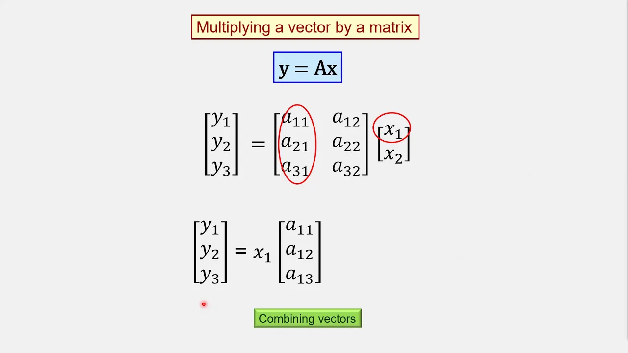
Vectors are containers of n numbers, depicted as arrows in 2-3D with elements as coordinate projections. The magnitude (norm) is the square root of sum of squared elements. A vector with magnitude 1 is a unit vector. Matrices are 2D containers with rows and columns, indexed by position. Matrix multiplication transforms vectors through linear operations: each output element is a weighted sum of input elements. This forms the foundation for linear algebra operations.
Click to watch →
Deep Dive
A conceptual understanding of what data is, including the difference between independent variables (features) and dependent variables (targets).

Manipulação de Dados em Python/Pandas - #01 Conceitos Básicos
28.1K
Variables in a dataset can be classified as independent or dependent. Independent variables (also called features, attributes, or input variables) exist without depending on other variables in the dataset. Dependent variables (also called target, output, or response variables) have dependencies on at least some of the independent variables. For example, in a fuel price dataset, state and unit of measure are independent variables, while the average resale price is a dependent variable because it is influenced by the state and other factors.
Click to watch →
Independent and Dependent Variables
651.8K
In scientific experiments, the independent variable (also called the manipulated variable) is the factor that is changed or controlled by the experimenter and can stand alone without being influenced by other variables; the dependent variable (also called the responding variable) is the outcome that is measured and changes in response to the independent variable. For example, when testing if car color affects interior temperature, the car color is the independent variable (what you change) and the temperature is the dependent variable (what you measure). When graphing these variables, the independent variable goes on the x-axis and the dependent variable on the y-axis, which can be remembered using the mnemonic DRY MIX (Dependent Responding Y-axis, Manipulated Independent X-axis).
Click to watch →

Identify Independent and Dependent Variables
255K
The independent variable is the factor that causes or determines changes in the dependent variable and always happens first; it is plotted on the x-axis of a graph. The dependent variable depends on or relies on the independent variable and cannot exist or change without it; it is plotted on the y-axis. To identify the independent variable in any situation, determine which variable must occur first for the other variable to matter or exist. For example, in the relationship between price and quantity sold, price is independent because it must be set before any sales can occur, while quantity sold is dependent because it changes based on the price.
Click to watch →

Independent vs Dependent Variables
41.7K
In algebra, an independent variable is a quantity that stands alone and doesn't rely on anything else to happen, while a dependent variable depends on or is affected by another variable; the independent variable typically happens first and is plotted on the x-axis, while the dependent variable follows and is plotted on the y-axis, and their relationship can show positive correlation (both increase together), negative correlation (one increases while the other decreases), constant correlation (remains unchanged), or no correlation.
Click to watch →
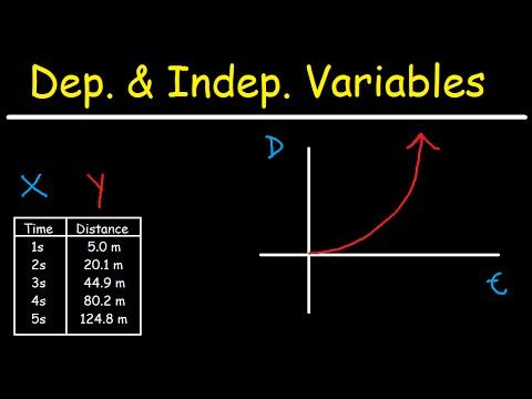
Dependent and Independent Variables
234.9K
In scientific experiments, the independent variable is the factor that is manipulated or controlled and is plotted on the x-axis, while the dependent variable is the outcome that is measured and plotted on the y-axis; for example, in Newton's second law (F=ma), mass is the independent variable and force is the dependent variable, resulting in a linear relationship where the slope equals acceleration, whereas in Boyle's law (PV=k), volume is the independent variable and pressure is the dependent variable, showing an inverse relationship, and in kinematics under constant acceleration, time is the independent variable and distance is the dependent variable, producing a quadratic or parabolic relationship described by d = (1/2)at².
Click to watch →
Prerequisite Knowledge
- Concept 01Basic Python programming syntax, including control flow, functions, and standard data structures like lists and dictionaries.
- Concept 02Familiarity with data manipulation and analysis libraries in Python, specifically Pandas and NumPy.
- Concept 03Fundamental mathematical concepts, particularly basic linear algebra (vectors and matrices) and introductory statistics (mean, median, standard deviation).
- Concept 04A conceptual understanding of what data is, including the difference between independent variables (features) and dependent variables (targets).
Subsequent Learning
- Step 01Advanced model evaluation and tuning techniques, such as k-fold cross-validation, grid search, and metrics like precision, recall, and F1-score.
- Step 02Feature engineering practices, including handling missing data, encoding categorical variables, and feature scaling/normalization.
- Step 03An introduction to Deep Learning and Artificial Neural Networks (ANNs) using frameworks like TensorFlow or PyTorch.
- Step 04Deploying machine learning models into production environments using web frameworks like Flask or FastAPI, or cloud platforms like AWS and Google Cloud.
Core Concepts
Journey Start
Core Concepts
0:06Playing Section
- 1
Explains machine learning purpose and real-world applications.
- 2
Covers key topics like modeling and algorithm evaluation.
- 3
Demonstrates use cases with facial and gesture recognition.
The Math-First Approach: Why Code-First Machine Learning Is Insufficient
While "code-first" courses using Python allow beginners to quickly build and deploy machine learning models, critics argue this approach fosters a superficial understanding of AI. By treating algorithms as "black boxes" via libraries like Scikit-Learn, learners often lack the foundational knowledge of linear algebra, calculus, probability, and mathematical statistics required to diagnose model failures, understand algorithmic bias, or innovate new architectures. This counterpoint emphasizes that genuine competence in machine learning requires a math-first foundation, warning that relying solely on Python APIs can lead to the misapplication of models, poor generalization to real-world data, and an inability to explain how decisions are made.
Deep Dive
Advanced model evaluation and tuning techniques, such as k-fold cross-validation, grid search, and metrics like precision, recall, and F1-score.

Scikit-Learn Crash Course: Python Machine Learning Library
647.4K
Proper model evaluation requires avoiding data leakage by using cross-validation, which splits data into multiple folds to ensure every point tests on unseen data. Grid search automates hyperparameter tuning by systematically trying combinations of parameters across cross-validation splits. Metric selection is critical: accuracy favors majority classes, while precision and recall trade off against each other depending on application costs. Custom metrics can be created using make_scorer() for domain-specific optimization. This rigorous evaluation methodology prevents overfitting and ensures models generalize well to production environments.
Click to watch →

الدكتور حليمي عبد الغفور - سلسلة الذكاء الاصطناعي التطبيقية ~ مقدمة في التعلم الآلي - 2025
10.2K
This section provides comprehensive coverage of model evaluation and hyperparameter tuning. The instructor demonstrates: (1) Using cross-validation (5-fold) instead of simple train-test split for more reliable evaluation; (2) Using classification reports and confusion matrices for classification models; (3) Using precision-recall curves and ROC curves for imbalanced datasets; (4) Using GridSearchCV and RandomizedSearchCV for automatic hyperparameter tuning; (5) Comparing different models (Random Forest vs. Gradient Boosting) using the same evaluation metrics. The instructor emphasizes that the best-performing model is not always the best choice - you must consider your specific problem and goals. The instructor demonstrates that Gradient Boosting achieved 84% accuracy compared to 82% for Random Forest, showing the value of trying different models and tuning hyperparameters.
Click to watch →

Scikit-Learn - 30 minutes, 30 commands, 80% of work done ! 🔥🔥🔥
28.5K
Cross-validation evaluates model performance by dividing data into multiple folds. In k-fold cross-validation, data is split into k subsets; for each iteration, k-1 folds train and 1 fold tests. The default is 5-fold. The cross_validate function returns scores across all folds. Hyperparameter tuning optimizes model performance: GridSearchCV exhaustively searches through specified parameter combinations, while RandomizedSearchCV randomly samples combinations for efficiency. Define parameter grid with ranges for each hyperparameter, specify iterations, and the function returns best parameters and corresponding score.
Click to watch →

Tutorial 3: Hand-Crafted Features and the Random Forest
301
For binary classification, accuracy alone is insufficient. Precision measures the proportion of predicted positives that are actually correct. Recall measures the proportion of actual positives correctly identified. F1 score is the harmonic mean of precision and recall. K-fold cross-validation (e.g., k=5) provides a more reliable estimate of model generalization by repeatedly splitting the data into training and validation sets. The results are averaged across folds. In the example, 5-fold cross-validation yielded an average accuracy of 62%, which is more reliable than a single train-test split.
Click to watch →

Scikit-Learn Full Crash Course - Python Machine Learning
56.6K
Cross-validation splits data into k folds, trains on k-1, evaluates on 1, repeating k times for reliable performance estimates. GridSearchCV systematically tries all hyperparameter combinations using cross-validation, returning best parameters and best estimator. This automates optimization of configuration settings like number of trees in random forest or depth of decision trees, improving model performance through systematic exploration of the hyperparameter space.
Click to watch →
Deep Dive
Feature engineering practices, including handling missing data, encoding categorical variables, and feature scaling/normalization.

Hands on Machine Learning - Chapter 2 - Full Machine Learning Project
145.1K
Data preparation for machine learning includes: (1) Feature engineering - creating new features from existing data using domain knowledge, (2) Imputation - handling missing values, (3) Encoding categorical variables, (4) Scaling numerical variables. Identify missing values using 'df.isnull().any()' and 'df.isnull().sum()'. Two basic approaches are dropping rows or columns with missing values, but imputation is often preferred. Use 'SimpleImputer(strategy='median')' to fill missing values with the median. For categorical variables, use ordinal encoding for ordered categories and one-hot encoding for nominal categories. One-hot encoding creates binary columns for each category, preventing the algorithm from incorrectly assuming category order.
Click to watch →
What is Feature Engineering | Feature Engineering Techniques | Feature Engineering | Intellipaat
4.5K
Feature engineering is the crucial machine learning preprocessing step that transforms raw data into structured features that algorithms can use to make predictions, involving techniques such as handling missing data through deletion or imputation (mean, median, mode), scaling continuous features via normalization (min-max scaling to 0-1 range) or standardization (z-score with mean 0 and unit variance), encoding categorical features using label encoding or one-hot encoding, and selecting relevant features through methods like variance threshold, chi-square test, recursive feature elimination, select from model, sequential feature selection, and correlation analysis to improve model performance, reduce complexity, and prevent overfitting.
Click to watch →
Feature Engineering Full Course - in 1 Hour | Beginner Level
36.6K
Feature engineering extracts more information from existing data to improve machine learning models. Two approaches exist: adding new external data and generating new features from existing data. Feature pre-processing transforms existing features through mathematical operations like log, square root, or reciprocal to handle non-linear relationships and skewness. Feature scaling normalizes different units using min-max scaling (0-1 range) or standard scaling (mean 0, std 1) for distance-based algorithms. Categorical variables require encoding: one-hot encoding converts categories to binary columns but loses order information for ordinal variables, while label encoding preserves order. For high-cardinality categories, sparse classes can be combined under an 'other' category to reduce dimensionality. The section demonstrates Python implementations using pandas and scikit-learn libraries on real datasets.
Click to watch →

Feature Engineering for Machine Learning| Cleaning | Encoding| Transformation | Scaling |AI with AI
170
Feature engineering is the process of transforming raw, unorganized data into features suitable for machine learning models. The five key steps are: (1) Data cleansing - removing errors, NaNs, and inconsistencies; (2) Data transformation - converting categorical data to numbers and scaling variables; (3) Feature extraction - creating new features from existing variables; (4) Feature selection - choosing the most relevant features; (5) Feature iteration - refining features based on model performance. The video demonstrates missing data handling using the Titanic dataset, showing how to check for missing values, drop rows with missing data, and implement imputation techniques including mean, median, and mode imputation. For categorical encoding, the video covers one-hot encoding (converting categorical data into binary variables), K-1 encoding (reducing columns by one to prevent multicollinearity), ordinal/label encoding (replacing categories with integers), count encoding (replacing categories with their frequency count), and frequency encoding (replacing categories with their percentage). The instructor demonstrates these using Titanic and Housing datasets with pandas functions like get_dummies() and map().
Click to watch →
Cleaning, Wrangling & Automation Guide 2026 | Data Pipelines in Python
283
Feature engineering creates new features (e.g., income per page) and bins numerical data using pandas.cut() with specified cut points. Encode categorical variables using OneHotEncoder or pandas.get_dummies, with drop_first=True to avoid multicollinearity. Scaling and normalization is critical for distance-based algorithms (nearest neighbor, SVM) where variables with different scales would dominate. Use StandardScaler to transform data to zero mean and unit variance.
Click to watch →
Deep Dive
An introduction to Deep Learning and Artificial Neural Networks (ANNs) using frameworks like TensorFlow or PyTorch.

Intro To Deep Learning With PyTorch - Deep Learning with Pytorch 1
133.4K
Deep learning is a subset of machine learning that uses neural networks—systems inspired by human brain neurons—to learn patterns from data through layers of interconnected nodes that process inputs, learn relationships, and produce outputs without requiring explicit programming for every possible scenario; PyTorch is a popular deep learning framework preferred over TensorFlow due to its Pythonic nature and ease of use, and this tutorial series will guide learners through setting up a development environment using Google Colab with GPU acceleration and GitHub integration to build and train neural networks for tasks like image classification and language modeling.
Click to watch →

Lecture 7: Introduction to TensorFlow
232.1K
Deep learning frameworks like TensorFlow enable rapid research iteration and democratize machine learning by providing automatic gradient computation, GPU acceleration, standardized interfaces, and access to pre-trained models. TensorFlow, developed by Google's Brain team, expresses machine learning as computational graphs where nodes represent operations and edges represent tensors (n-dimensional arrays). This graph-based paradigm simplifies building complex models from simple operations and enables automatic differentiation for gradient calculations.
Click to watch →

3MTT Onboarding and Learning Walkthrough Call
20.5K
TensorFlow and PyTorch are open-source deep learning frameworks used for building and training artificial neural networks. They provide high-level APIs for constructing, training, and deploying machine learning models, particularly for deep learning applications. Key features include automatic differentiation for efficient gradient computation, support for structured data, images, text, and time series, and a wide range of pre-built layers and activation functions. These frameworks are used for tasks like image classification, transformer models, NLP, and text generation.
Click to watch →

Frameworks de Machine Learning | TensorFlow, Pytorch, Keras
3.1K
TensorFlow is the most widely-used machine learning framework for artificial intelligence, particularly for deep learning applications. It supports development on Windows and enables projects involving neural networks. Deep learning networks differ from shallow neural networks by having multiple layers, allowing them to recognize voice, images, and various applications. PyTorch is another framework used by major companies like Facebook, though it has less documentation and fewer shared projects compared to TensorFlow. Both frameworks enable classification tasks where AI learns to categorize objects based on training data.
Click to watch →
Семинар. Введение в PyTorch
16.2K
PyTorch is one of the most popular deep learning frameworks today, chosen for its convenience, informative documentation, and widespread adoption. The evolution of deep learning frameworks includes early frameworks like Caffe, Theano, and Lasagne (now outdated), TensorFlow (popular until 2017-2018 but complex to use), and Keras (a simpler wrapper but less flexible). PyTorch emerged in 2017-2018 as a more convenient alternative that resembles working with NumPy. The fundamental data structure in PyTorch is the tensor, which is analogous to NumPy arrays and serves as the basis for all neural network computations.
Click to watch →
Deep Dive
Deploying machine learning models into production environments using web frameworks like Flask or FastAPI, or cloud platforms like AWS and Google Cloud.

How To Deploy A Machine Learning Model On AWS EC2 | AUG 2021 Updated | ML Model To Flask Website
106.6K
This tutorial demonstrates how to deploy a machine learning model as a web application using Flask framework and host it on AWS EC2 cloud platform. The process involves: (1) Building and training an ML model (using student placement prediction as example), (2) Exporting the trained model using pickle library, (3) Creating a Flask web application with HTML forms for user input, (4) Setting up AWS EC2 instance with Ubuntu OS, (5) Configuring security groups and SSH access, (6) Uploading project files to EC2 using WinSCP, (7) Installing dependencies via pip and requirements.txt, (8) Running the Flask app using nohup command to keep it running continuously. The complete workflow transforms a standalone ML model into an accessible web service that can be accessed globally through the internet.
Click to watch →

NLP Pipeline: NLP Tutorial For Beginners In Python - S1 E6
105.9K
Deployed models are exported to files and hosted on cloud platforms (AWS, Azure, Google Cloud). Services like FastAPI or Flask create REST APIs that accept HTTP requests and return predictions. End-to-end ML platforms like Databricks, Amazon SageMaker, Azure Machine Learning, and H2O.ai provide integrated environments for building, deploying, and managing production ML services.
Click to watch →
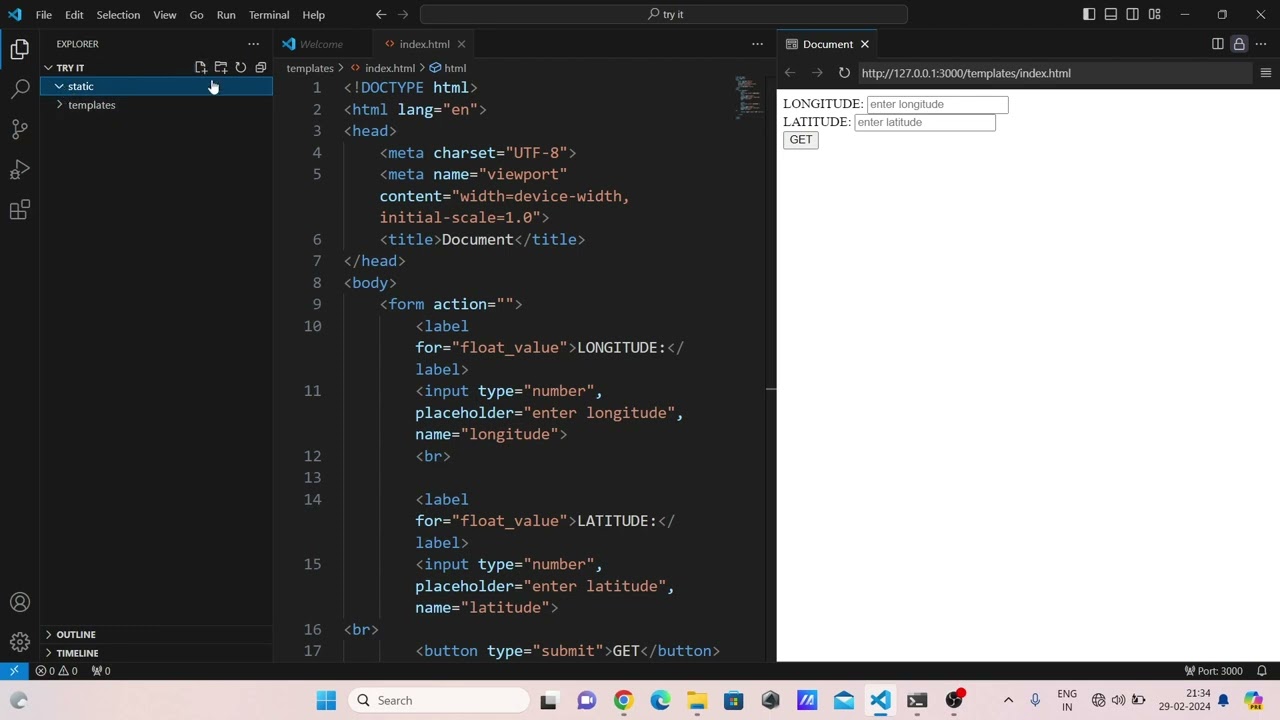
48 Deploy Machine Learning Model using Flask part 1
537
To make a machine learning model accessible to everyone, it needs to be deployed to a production server. The instructor explains that the development server is only for local testing. Production deployment involves hosting the application on a Virtual Private Server (VPS) or cloud platform. The instructor mentions services like AWS, Google Cloud, and Microsoft Azure that provide cloud computing resources. These platforms allow the application to be accessible via the internet and can handle multiple simultaneous requests. Cloud platforms offer various services including computational resources, database services, storage services, and AI/ML services. These services can be used to host machine learning models and make them accessible to users worldwide.
Click to watch →
38 Data Science Tools For Beginners to Experts
2.4K
Deploying machine learning models requires web application frameworks like Flask (lightweight micro framework) and Django (complex system with built-in features). Cloud platforms enable model hosting and scalability: AWS is the most widely used cloud system, Google Cloud Platform offers native AI and ML tools, Microsoft Azure provides enterprise support, PythonAnywhere specializes in Python hosting, and Heroku simplifies deployment without learning complex cloud infrastructure. Understanding deployment is essential for data scientists to move models from development to production environments.
Click to watch →
Deploying Machine Learning Models with FastAPI, Docker, and AWS ECS: A Step-by-Step Guide
81.9K
Deploying machine learning models into production requires a three-step strategy: (1) wrapping the model in an API using FastAPI to enable programmatic access, (2) containerizing the API with Docker to package all dependencies into a portable image, and (3) deploying the container on cloud infrastructure like AWS Elastic Container Service. This approach transforms a standalone machine learning model into a scalable, accessible solution that can be integrated into websites, mobile applications, or business processes.
Click to watch →
Core Concepts
Journey Start
Core Concepts
0:06- 1
Explains machine learning purpose and real-world applications.
- 2
Covers key topics like modeling and algorithm evaluation.
- 3
Demonstrates use cases with facial and gesture recognition.
The Math-First Approach: Why Code-First Machine Learning Is Insufficient
While "code-first" courses using Python allow beginners to quickly build and deploy machine learning models, critics argue this approach fosters a superficial understanding of AI. By treating algorithms as "black boxes" via libraries like Scikit-Learn, learners often lack the foundational knowledge of linear algebra, calculus, probability, and mathematical statistics required to diagnose model failures, understand algorithmic bias, or innovate new architectures. This counterpoint emphasizes that genuine competence in machine learning requires a math-first foundation, warning that relying solely on Python APIs can lead to the misapplication of models, poor generalization to real-world data, and an inability to explain how decisions are made.
Basic Python programming syntax, including control flow, functions, and standard data structures like lists and dictionaries.
Familiarity with data manipulation and analysis libraries in Python, specifically Pandas and NumPy.
Fundamental mathematical concepts, particularly basic linear algebra (vectors and matrices) and introductory statistics (mean, median, standard deviation).
A conceptual understanding of what data is, including the difference between independent variables (features) and dependent variables (targets).
Advanced model evaluation and tuning techniques, such as k-fold cross-validation, grid search, and metrics like precision, recall, and F1-score.
Feature engineering practices, including handling missing data, encoding categorical variables, and feature scaling/normalization.
An introduction to Deep Learning and Artificial Neural Networks (ANNs) using frameworks like TensorFlow or PyTorch.
Deploying machine learning models into production environments using web frameworks like Flask or FastAPI, or cloud platforms like AWS and Google Cloud.
35.2K views199likes2:22@CognitiveClassOriginal Release: 2017-03-07
hello and welcome to machine learning with python in this course we'll be reviewing two main components first you learning about the purpose of machine learning and where it applies in the real world second you'll get a general overview of machine learning topics such as statistical modeling supervised vs unsupervised learning model evaluation and machine learning algorithms and clustering there are many technologies that integrate machine learning many of which you may use in your daily life a great example of this is snapchat in which its facial recognition is an example of machine learning machine learning is also used in Xbox Kinect which projects an infrared grid to determine depth movement and body shape of one or more people gesture recognition is used to analyze that data and output the results into the game machine learning impact Society in a very influential way here are some real life examples how do you think netflix and youtube recommend videos movies and TV shows to their users they use machine learning to produce suggestions that you might enjoy this is similar to how your friends might recommend to show to you based on other shows you've watched IBM Watson uses machine learning algorithms to do almost anything including things like helping doctors identify cancer treatments it's also been used in developing early childhood education models there's virtually no end to what IBM Watson can do thanks to machine learning together data is gathered to train a machine learning model so we can understand patterns within the data once the model has been trained it can be used to predict the results of out-of-sample data or data in which the results are unknown collectively this is how machine learning is achieved so now that you have a sense of what's in store on this journey let's get started with machine learning thanks for watching and remember by completing the course you'll be one step closer to earning a badge with all the benefits that come with it
Up Next

16:28
Time Series Forecasting in Python: Implementing ARIMA Models End-to-End
@UnfoldDataScience
53.7K views•2020-12-16

57:48
Secure Multiparty Computation (MPC): Foundations & Challenges
@SimonsInstitute
7.3K views•2015-05-28

13:03
Bypassing Tor Censorship: Bridges and Pluggable Transport Guide
@Coding_ForEveryone
397 views•2024-06-11

18:41
Neural Networks Explained: Math, Layers, and Learning Fundamentals
@3blue1brown
21.9M views•2017-10-05
Related Study Plans & Knowledge Roadmaps
Structured learning paths in Artificial Intelligence
artificial-intelligence
Aligning LLMs: DPO, TRL & Custom Datasets
01Foundations of Python & Machine Learning
02Transformers and Large Language Models (LLMs)
03Aligning LLMs: SFT and RLHF
+ 3 more learning modules
24h6 modules
Explore Roadmap
artificial-intelligence
Federated Learning: PyTorch, Flower & Privacy
01Python & Machine Learning Foundations
02Deep Learning Basics with PyTorch
03Introduction to Federated Learning
+ 2 more learning modules
35h5 modules
Explore Roadmap
artificial-intelligence
Securing LLMs: Guardrails AI & NeMo Gateway
01Introduction to LLMs, Python, and APIs
02Understanding LLM Vulnerabilities & Threats
03Defending LLMs with Guardrails AI
+ 2 more learning modules
15h5 modules
Explore Roadmap
artificial-intelligence
Building Recommenders: Two-Tower & Vector DBs
01Foundations of Python & Machine Learning Basics
02Introduction to Recommender Systems
03Deep Learning & Representation Learning
+ 3 more learning modules
75h6 modules
Explore Roadmap