This workshop introduces two essential model interpretability techniques—LIME and SHAP—for data scientists working with complex machine learning models. The focus is on practical application in Python using a real-world data science problem, emphasizing why interpretability matters even when models are highly sophisticated. LIME (Local Interpretable Model-agnostic Explanations) and SHAP (SHapley Additive exPlanations) are presented as critical tools to understand and explain model predictions, making them indispensable in professional data science workflows. The session is part of PyData NYC 2018, an event organized by NumFOCUS that supports the global data science community through educational content and community-driven learning. The workshop aims to equip attendees with actionable methods to demystify black-box models, ensuring transparency and trust in machine learning outcomes. While the description does not detail specific algorithms or mathematical foundations, it clearly positions LIME and SHAP as core techniques that should be in every data scientist’s toolkit. The presentation is designed for practical adoption, not theoretical exploration, and assumes familiarity with basic machine learning concepts. The context of PyData indicates a focus on real-world implementation using open-source tools, particularly in Python.
Model Interpretability with LIME & SHAP | Data Science Tutorial
Added:Fundamental understanding of supervised machine learning concepts, including classification, regression, and ensemble methods like Random Forests or Gradient Boosting.

Random forest is an ensemble method using bootstrap aggregation (bagging) that trains multiple decision trees on random data and feature subsets, reducing variance and overfitting. Gradient boosting builds trees sequentially where each tree corrects errors from previous ones using loss function gradients, focusing on reducing bias. Bagging trains trees in parallel while boosting trains them sequentially with error correction.

Supervised machine learning involves learning a function that maps input features to output labels from training data, with two primary approaches: regression for continuous outputs using linear models with optimization techniques like gradient descent and regularization (L1/L2), and classification for discrete outputs using algorithms like logistic regression, support vector machines, and decision trees; ensemble methods such as bagging (random forests) and boosting (AdaBoost) combine multiple models to improve prediction performance by reducing variance and bias respectively.

Supervised learning encompasses classification (predicting discrete categories) and regression (predicting continuous values). Classification includes multi-class and binary problems. Regression uses linear models with Lasso (L1 regularization) for feature selection and Ridge (L2 regularization) for overfitting prevention. Logistic regression applies linear principles to classification using sigmoid functions and maximum likelihood. Softmax extends this to multi-class classification. Ensemble learning combines multiple models: decision trees use recursive partitioning with pruning; bagging creates parallel models on bootstrap samples; random forest adds feature randomness; boosting builds models sequentially with AdaBoost focusing on difficult examples and gradient boosting using gradient descent optimization.

Ensemble methods combine multiple machine learning models to create more powerful models. Random Forest and Gradient Boosted Decision Trees are two ensemble methods that dominate machine learning competitions. Random Forest addresses the main drawback of decision trees—overfitting—by combining many slightly different decision trees. Each tree is trained on a different subset of data and features, then their results are averaged to reduce overfitting while maintaining predictive power.

Supervised learning includes classification (predicting discrete categories) and regression (predicting continuous values). Classification algorithms include Logistic Regression for binary outcomes, Support Vector Machines for finding optimal decision boundaries, K-Nearest Neighbors for neighbor-based labeling, and Decision Trees for hierarchical feature-based splitting. Regression algorithms include Linear Regression for linear relationships, Polynomial Regression for complex patterns, and Ridge/Lasso Regression with regularization to prevent overfitting. Ensemble methods combine multiple models: Random Forest (bagging) averages many decision trees, while Boosting iteratively improves weak learners, with XGBoost being particularly popular in industry applications.
Familiarity with standard model evaluation metrics (e.g., accuracy, precision, recall, F1-score, and ROC-AUC) to understand what the models are optimizing.
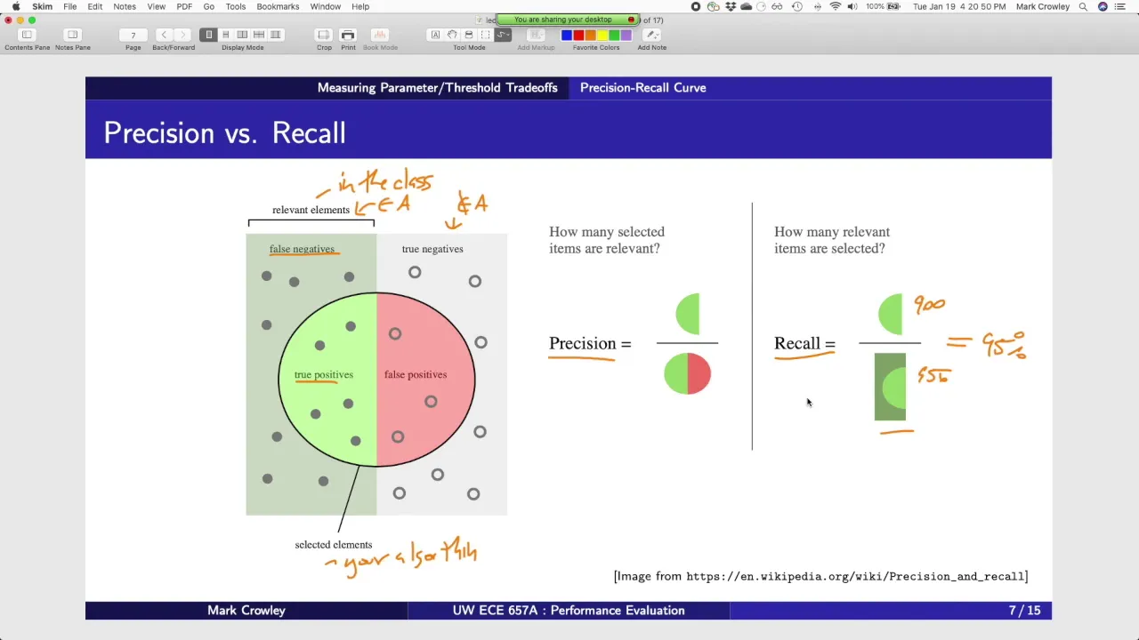
Beyond basic accuracy (correct predictions divided by total predictions), multiple specialized metrics address different failure modes. Precision focuses on trustworthiness of positive identifications, recall emphasizes capturing all relevant cases, and the F1 score combines both using harmonic mean to ensure neither metric is sacrificed entirely. These metrics are weighted differently across domains—medical screening prioritizes recall to avoid missing cases, while spam filtering prioritizes precision to minimize false alarms. The choice of evaluation metric fundamentally shapes what models optimize for, making domain expertise essential for effective model deployment.
![Python Curso Completo [2024]](https://i.ytimg.com/vi_webp/PYfcybsw9LM/maxresdefault.webp)
Common metrics for evaluating classification models include: accuracy (overall correctness), precision (correct positive predictions), recall (correct negative predictions), F1 score (harmonic mean of precision and recall), and ROC-AUC (measures model performance across different thresholds). These metrics help understand different aspects of model performance.

Classification metrics include: Accuracy = (TP+TN)/(TP+TN+FP+FN) for overall correctness; Precision = TP/(TP+FP) for avoiding false positives (use when legitimate items incorrectly flagged is costly); Recall = TP/(TP+FN) for catching all positives (use in medical diagnosis); F1 score = 2×(precision×recall)/(precision+recall) for balanced measure; ROC-AUC measures model's ability to rank predictions across thresholds, useful for imbalanced datasets. Choose metrics based on what errors are most costly: precision for avoiding false positives, recall for catching all positives, F1 for balance, ROC-AUC for ranking ability.

Machine learning metrics measure algorithm quality: for classification, accuracy (correct predictions/total), precision (true positives/predicted positives), recall (true positives/actual positives), F1 score (harmonic mean of precision and recall), and ROC-AUC (area under receiver operating characteristic curve); for regression, MSE (mean squared error) and MAE (mean absolute error). Metric selection depends on task goals, with ROC-AUC being particularly valuable for imbalanced datasets as it remains unaffected by class distribution.

The ROC (Receiver Operating Characteristic) curve plots True Positive Rate against False Positive Rate at various probability thresholds. A perfect model hugs the top-left corner (AUC = 1), while random guessing follows the diagonal (AUC = 0.5). Higher AUC indicates better class separation. Model accuracy is a subset of overall performance - in imbalanced datasets like fraud detection, high accuracy can be misleading because the model might simply predict the majority class. Other metrics like precision, recall, F1 score, and AUC-ROC should be considered for comprehensive evaluation.
Basic knowledge of feature importance concepts and how traditional machine learning algorithms inherently rank feature significance.

Feature importance measures how much each input variable contributes to a model's predictions. Some models like Random Forest provide built-in feature importances via .feature_importances_ after training. The process involves: (1) loading data and performing train-test split, (2) fitting the classifier on training data, (3) accessing importances, (4) zipping with feature names to create a dictionary, and (5) sorting in descending order. This allows practitioners to identify which features drive decision-making in the model.

Model-based feature importance uses trained machine learning models to assess predictor contributions. Linear regression coefficients indicate sensitivity, but beta coefficients solve scale dependency by standardizing all features to mean 0 and variance 1. Tree-based models like random forests provide direct feature importance scores. Recursive feature elimination iteratively builds models, identifies least important features (lowest absolute coefficient/importance), removes them, and rebuilds until desired features remain. This produces complete rankings from most to least important. RFE advantages include consistency with final model type and flexibility to use any model providing feature importance. Different models (linear regression vs random forests) may produce different rankings due to varying flexibility. The choice of methodology impacts feature importance assessment, and comparing multiple approaches provides more reliable insights into feature relevance.

Feature importance measures which variables contribute most to predictive accuracy. One approach involves permuting (shuffling) each feature's values and measuring the resulting increase in prediction error. If shuffling a feature significantly degrades performance, that feature is important; if shuffling has minimal effect, the feature is unimportant. This provides interpretability similar to p-values in traditional statistics but through a different computational mechanism.

Feature importance is calculated by measuring the decrease in model performance when each feature is randomly shuffled. The process: train a random forest, calculate baseline performance, shuffle each feature, measure performance drop, and the drop indicates importance. This method works for any model type, not just random forests, and is computationally efficient compared to retraining models. Higher importance values indicate more predictive power. This allows prioritizing investigation of the most important features.

Feature importance is calculated through a systematic algorithm: First, identify all nodes in the tree where each feature is used. For each such node, calculate the proportion of observations from the original data. Measure the impurity of the node and its child nodes. Calculate importance at each node as the weighted difference between parent impurity and the sum of child impurities, normalized by 100. Total feature importance is the sum of importances calculated at each node where the feature was used, divided by the total importance of all features. This algorithm reveals that feature importance values can differ based on which quality measure (splitting criterion) is chosen for tree construction, making it important to understand which criterion is being used when interpreting feature importance.
Proficiency in Python programming, particularly using data science libraries such as Scikit-Learn, Pandas, and NumPy.

Five essential Python libraries for data science: (1) Numpy (Numerical Python) is the core library for scientific computations with n-dimensional arrays for linear algebra and random-number generation; (2) Matplotlib is a plotting library for 2D graphics used in scripts, shells, and web applications; (3) Pandas is used for data manipulation, analysis, and cleaning of tabular, time series, and observational data; (4) Seaborn is based on matplotlib for statistical visualization with multi-plot grids and automatic regression estimation; (5) Scikit-learn is an open-source machine learning library providing supervised and unsupervised learning algorithms.
![Data Science Full Course | Complete Data Science Full Course For Beginners IBM [PART 7]](https://i.ytimg.com/vi/JCix5j4OdWI/maxresdefault.jpg)
Python is the preferred language for data scientists. Key libraries include: NumPy for efficient computation with n-dimensional arrays; SciPy for numerical algorithms in signal processing, optimization, and statistics; Matplotlib for 2D and 3D plotting; Pandas for high-performance data structures with functions for importing, manipulating, and analyzing data; Scikit-learn for machine learning algorithms including classification, regression, and clustering. Scikit-learn implements the entire machine learning pipeline including data pre-processing, feature selection, train-test splitting, defining algorithms, fitting models, tuning parameters, prediction, evaluation, and exporting models. The entire process can be done in a few lines of code, making it accessible for beginners.

Key Python libraries for data science include: Pandas (for data manipulation), NumPy and SciPy (for numerical computing and matrix operations), Matplotlib (for visualization), Seaborn (for easier visualization), IPython (for interactive environments), Jupyter Notebooks (for documentation and sharing), and scikit-learn (for machine learning). Understanding the underlying libraries like NumPy and SciPy is important as they form the basis for many other tools.

This tutorial demonstrates the complete workflow for training and testing regression models using Scikit-Learn, including data preparation (converting Pandas DataFrames to NumPy arrays), feature and label separation, data scaling for improved accuracy, cross-validation for unbiased training/testing splits, and model evaluation using accuracy metrics. The video shows how to implement Linear Regression and Support Vector Regression, highlighting the importance of using separate training and testing datasets to prevent overfitting, and demonstrates how different algorithms can yield significantly different results (96% vs 51% accuracy in the example).

This comprehensive section covers three essential Python libraries for data science. Matplotlib enables data visualization through line plots, bar charts, scatter plots, and area plots using functions like plt.plot(), plt.bar(), plt.scatter(), and plt.fill_between(). NumPy provides numerical computing capabilities with array creation (np.array()), operations (np.sum(), np.mean(), np.min(), np.max()), reshaping (np.reshape()), and random generation (np.random.randint()). Pandas handles data manipulation with DataFrames created from dictionaries, CSV import/export (.to_csv(), .read_csv()), and statistical analysis (.head(), .tail(), .info(), .describe()). These libraries form the foundation for data analysis, visualization, and manipulation in Python programming.
An introductory awareness of the 'black-box' nature of complex models and the trade-off between model accuracy and interpretability.

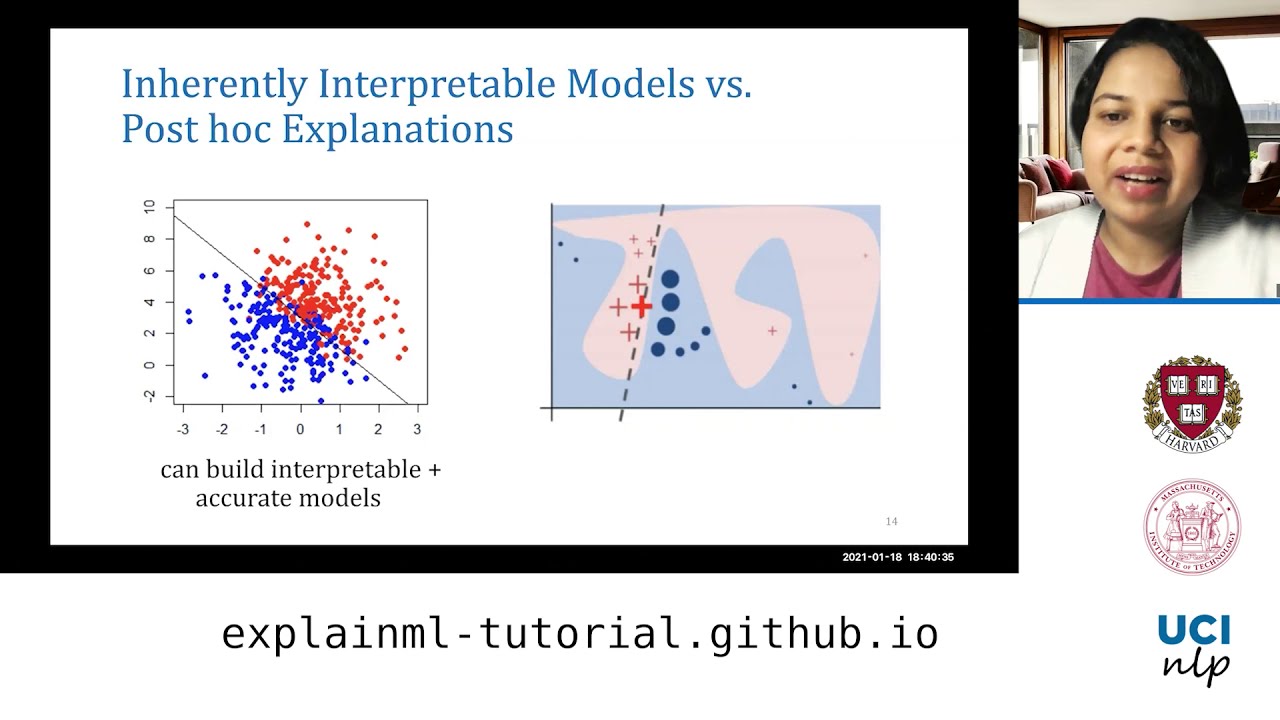
A fundamental trade-off exists between model interpretability and predictive accuracy. Inherent interpretability comes at the cost of potential accuracy limitations, while complex models achieve higher accuracy but sacrifice transparency. This trade-off emerges when data becomes more complex, high-dimensional, and large-scale—as seen in natural language processing, computer vision, and biomedical datasets. When simple models cannot achieve adequate accuracy for complex tasks, practitioners must choose between accepting lower accuracy with interpretability or using complex models with post-hoc explanations. Additionally, situations with insufficient data for building models from scratch force reliance on post-hoc explanations for proprietary black-box models.

There is a fundamental trade-off between accuracy and interpretability in modeling tools. A model that takes in more factors and adds more weights can produce more accurate results but becomes harder to understand, harder to pick apart, and harder to think about. A model with too much unexplained complexity becomes a black box that users must blindly trust, which is unreasonable to ask. It's better to have an imperfect but somewhat simpler model that people can open the hood on and check out the inner workings before deciding how to consider its outputs.
![12.1 Model Interpretation Motivation [Applied Machine Learning || Varada Kolhatkar || UBC]](https://i.ytimg.com/vi/xfICsGL7DXE/maxresdefault.jpg)
In machine learning, there is a fundamental trade-off between model accuracy and interpretability: simple models like logistic regression are highly interpretable through feature coefficients but may sacrifice accuracy, while complex models like XGBoost and LightGBM achieve higher accuracy but become less interpretable; this trade-off is particularly critical in high-stakes domains such as banking, healthcare, and criminal justice where understanding model decisions is essential for diagnosing systematic errors and biases.

In machine learning, there is a fundamental trade-off between prediction accuracy and model interpretability: flexible models (like thin plate splines, bagging, boosting, SVM, and deep learning) can closely follow the true function and achieve higher prediction accuracy but are difficult to interpret, while restrictive models (like linear regression and LASSO) are more interpretable but may miss complex patterns in the data. The choice between them depends on the goal—use flexible models when prediction accuracy is paramount (e.g., stock price forecasting) and restrictive models when understanding the relationship between predictors and response is important (e.g., understanding how education years and seniority affect income).

Neural networks, while powerful for tasks like image recognition (achieving 95% accuracy), function as 'black boxes' where the internal decision-making process is opaque and difficult to interpret. This lack of transparency can lead to unexpected failures, such as when a military vehicle detection system learned to detect darkness rather than military vehicles, or when a husky was misclassified as a wolf because the network focused on background patterns. These limitations have prompted researchers to explore explainable AI (XAI) and traditional algorithmic approaches that provide clearer, more interpretable decision rules, even if they achieve slightly lower accuracy (94% vs 95%).
Prerequisite Knowledge
- Concept 01Fundamental understanding of supervised machine learning concepts, including classification, regression, and ensemble methods like Random Forests or Gradient Boosting.
- Concept 02Familiarity with standard model evaluation metrics (e.g., accuracy, precision, recall, F1-score, and ROC-AUC) to understand what the models are optimizing.
- Concept 03Basic knowledge of feature importance concepts and how traditional machine learning algorithms inherently rank feature significance.
- Concept 04Proficiency in Python programming, particularly using data science libraries such as Scikit-Learn, Pandas, and NumPy.
- Concept 05An introductory awareness of the 'black-box' nature of complex models and the trade-off between model accuracy and interpretability.
Subsequent Learning
- Step 01In-depth study of Cooperative Game Theory, specifically the mathematical axioms behind Shapley values which form the foundation of SHAP.
- Step 02Exploration of advanced interpretability methods for deep learning, such as Integrated Gradients, Layer-wise Relevance Propagation (LRP), and Grad-CAM for computer vision.
- Step 03Implementation of Counterfactual Explanations and Anchors to provide actionable recourse for users affected by algorithmic decisions.
- Step 04Application of model interpretability tools in AI Ethics and Governance to detect model bias, audit algorithmic fairness, and comply with regulations like GDPR's 'right to explanation'.
- Step 05Deployment of LIME and SHAP in production environments for real-time model monitoring, debugging, and explaining model predictions to non-technical stakeholders.
Interpretability Intro
4:01- 1
Explains why model interpretability is crucial for trust and debugging.
- 2
Highlights risks of black-box models using real-world examples of bias.
The Fallacy of Post-Hoc Explanations (Inherently Interpretable Models)
While LIME and SHAP are widely used to explain complex 'black-box' models, prominent researchers argue that post-hoc explanations are fundamentally flawed, especially for high-stakes decisions. First, these methods only approximate the model's behavior, meaning the explanations themselves can be inaccurate, highly unstable, or easily manipulated. Second, they can create a false sense of security by masking biased underlying logic. This counter-perspective advocates for using 'inherently interpretable' models—such as decision trees, rule lists, or generalized additive models—from the start, eliminating the need for unreliable approximations.
In-depth study of Cooperative Game Theory, specifically the mathematical axioms behind Shapley values which form the foundation of SHAP.

The Shapley value provides a systematic method for fairly allocating the value generated by coalitions in cooperative games, based on four foundational axioms: efficiency (total payoff equals coalition value), symmetry (equally contributing players receive equal payoffs), the null player axiom (players who contribute nothing receive nothing), and additivity (payoffs are consistent across different games). These axioms ensure equitable distribution of coalition gains by considering all possible coalition structures and each player's marginal contribution across different coalition formations.

Shapley values provide a mathematically rigorous method for fairly distributing the total value of a cooperative game among its players by calculating each player's expected marginal contribution—the weighted average of their contribution to all possible coalitions they could join—where the weights are determined by the probability of each coalition forming, derived from the number of ways players can sequentially join coalitions; this fairness is guaranteed by satisfying four key axioms: efficiency (all value is distributed), symmetry (identical contributors receive equal shares), null player (players contributing nothing receive nothing), and additivity (contributions combine across independent games).

This section derives SHAP values from cooperative game theory, originally developed by Lloyd Shapley in the 1950s. The core problem is fairly distributing a total payoff among players who contributed differently, with Shapley proving that only one unique solution satisfies fairness properties: additivity and consistency. The mathematical formulation defines SHAP values as the average marginal contribution of a feature across all possible feature subsets—calculating model outputs with and without each feature, then averaging differences. This theoretical foundation ensures SHAP provides the only mathematically unique solution for fair feature attribution. The section explains why this matters: without such a theoretical guarantee, different explanation methods could produce arbitrarily different results, undermining trust in model interpretability tools.

The Shapley Value is a solution concept in cooperative game theory that fairly divides the total value generated by a coalition among its members by calculating each member's average marginal contribution across all possible coalition formation orders, satisfying three key axioms: symmetry (identical contributors receive identical payoffs), dummy player (non-contributors receive nothing), and additivity (value allocation separates cleanly across independent games).

Cooperative game theory addresses how to divide gains or costs fairly among collaborating players using the Shapley Value method. This approach satisfies four axioms: marginal contribution determines each player's value based on what is gained by removing them; interchangeable players receive equal value; dummy players who contribute nothing receive nothing; and costs should be decomposed across different parts of the game. Applying this to a cookie-baking example where one person produces 10 cookies/hour and another 20 cookies/hour, but together they produce 40 cookies/hour, the Shapley Value calculates each person's fair share by averaging their marginal contributions to the coalition. This method ensures equitable distribution while accounting for individual contributions, and scales to complex coalitions with many participants.
Exploration of advanced interpretability methods for deep learning, such as Integrated Gradients, Layer-wise Relevance Propagation (LRP), and Grad-CAM for computer vision.

White-box methods require model access to compute explanations. Grad-CAM (Gradient-weighted Class Activation Mapping) generates heatmaps using activations from the last convolutional layer and gradient computations to highlight important image regions. Layer-wise Relevance Propagation (LRP) propagates information backward through network layers using layer-specific rules, providing higher resolution explanations than Grad-CAM. Both methods suffer from low resolution due to the last convolutional layer's limited spatial detail. Evaluation against human fixation data shows some methods produce heatmaps more aligned with human visual attention patterns, though resolution limitations persist.

Gradient-based attribution methods compute feature importances using backpropagation techniques. DeepLift addresses gradient saturation issues by computing attributions relative to reference values rather than infinitesimal changes. Grad-CAM and similar methods calculate gradients of loss with respect to input features, producing salient region heatmaps for images. Integrated Gradients improves robustness by computing gradients along paths between inputs and baselines, then integrating results. These methods leverage neural network gradients to provide computationally efficient explanations while maintaining theoretical grounding.

Layer-wise Relevance Propagation (LRP) is a structure-based explanation method for deep neural networks that decomposes classification predictions by redistributing relevance values backward through the network layers, using neuron activations and connection weights to determine which input features contributed most to the prediction; unlike gradient-based methods that suffer from local sensitivity and gradient shattering problems in deep networks, LRP leverages the hierarchical structure of neural networks to provide more reliable and interpretable explanations, and can be extended to explain various machine learning models including clustering algorithms through a numericalization trick.
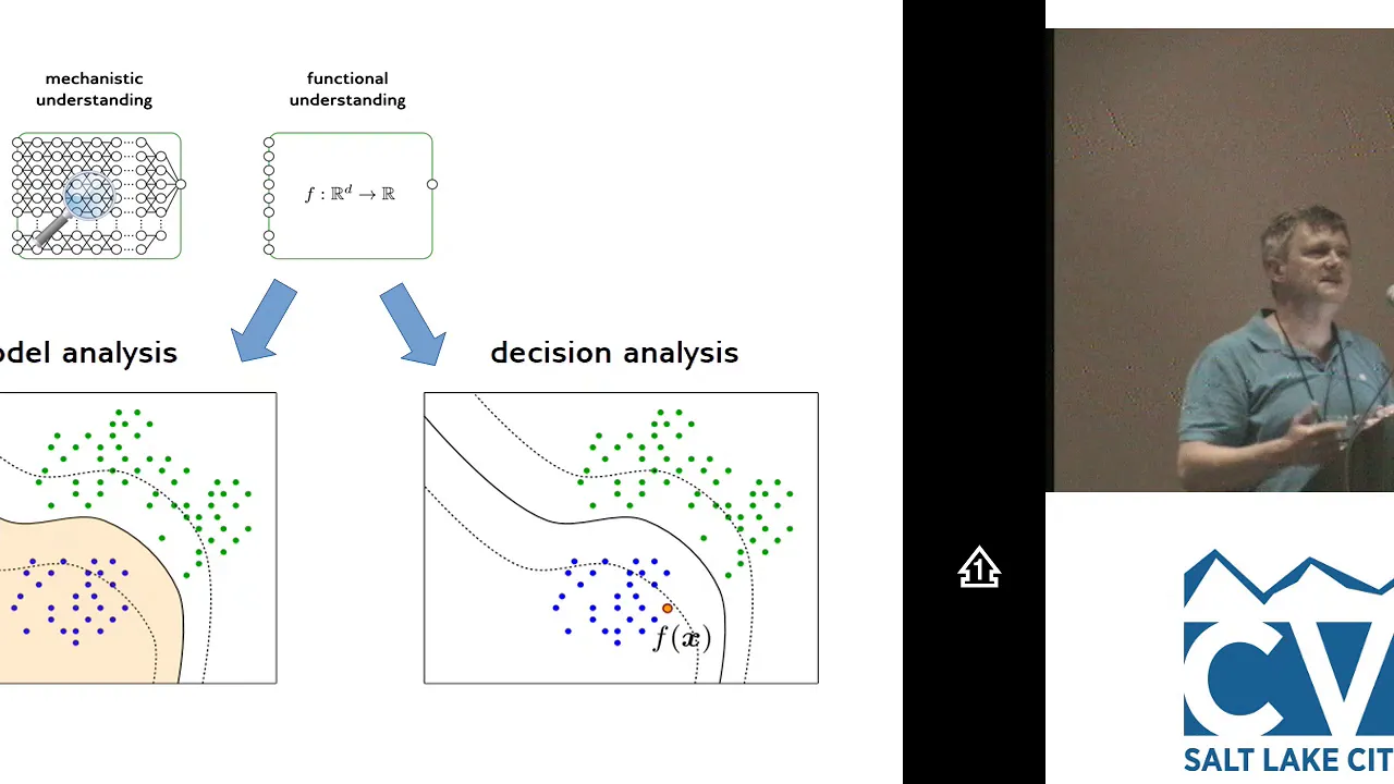
Layer-wise Relevance Propagation (LRP) is a model-agnostic technique for interpreting deep neural networks by decomposing classification decisions into pixel-level relevance scores, which addresses fundamental limitations of gradient-based sensitivity analysis such as gradient shattering and discontinuity issues; unlike sensitivity analysis that explains prediction variation, LRP explains the prediction itself by propagating relevance backward through network layers using mathematical rules derived from Taylor decomposition, ensuring conservation, continuity, and selectivity properties that make it superior for understanding model behavior in applications ranging from computer vision to natural language processing.

Grad-CAM (Gradient Class Activation Mapping) is a technique for explaining computer vision model predictions. Explainable machine learning addresses why models make predictions by examining data features, feature relationships, and model patterns. Three dimensions of interpretability exist: data features, feature relationships, and model patterns. While there's a traditional trade-off between model accuracy and interpretability, techniques like Grad-CAM enable both. Resources include books like 'Interpretable Machine Learning' and repositories from Microsoft and IBM.
Implementation of Counterfactual Explanations and Anchors to provide actionable recourse for users affected by algorithmic decisions.
Counterfactual explanations provide actionable recourse by identifying minimal feature changes needed to flip a model's prediction. Early methods minimized distance between original and modified instances but could suggest unrealistic changes (changing race/gender). Modern approaches incorporate user-specified constraints and use cost functions accounting for feature interactions. These explanations help affected individuals understand how to potentially reverse unfavorable decisions, such as suggesting salary increases or debt reduction to obtain loan approval.

Counterfactual explanations provide recourse recommendations to users negatively affected by machine learning decisions. They represent minimal input changes needed to flip model predictions from negative to positive outcomes. The mathematical formulation involves optimizing a loss function balancing validity (correct prediction flip) against distance minimization (effort required). However, this basic formulation creates fundamental robustness challenges, as minimizing distance causes counterfactuals to concentrate precisely at decision boundaries—positions inherently vulnerable to instability.

Counterfactual explanations answer the question: what changes to features would flip a model's prediction? This concept is crucial for applications like loan approvals, where denied applicants deserve actionable guidance. The minimum distance approach finds the closest instance x' to original x that achieves the desired outcome, requiring gradient access. Advanced methods incorporate ethical constraints by defining feasible sets excluding sensitive attributes, and account for practical feature costs. Structural causal models ensure generated counterfactuals respect real-world relationships, while variational autoencoders generate realistic examples in latent spaces. These techniques enable fair recourse recommendations while preventing harmful suggestions like changing protected attributes.

Algorithmic recourse provides actionable steps for individuals to reverse unfavorable algorithmic decisions, distinguishing it from counterfactual explanations which merely describe hypothetical scenarios. While counterfactual explanations assume independent feature manipulation, algorithmic recourse requires accounting for causal relationships between features to ensure proposed actions will actually achieve the desired outcome. Complete causal knowledge is theoretically necessary to guarantee effective recourse, but practical implementations must relax these assumptions using probabilistic approaches due to the impossibility of obtaining perfect causal models in real-world applications.

Algorithmic recourse addresses providing recommendations to users negatively affected by ML model decisions. Counterfactual explanations are minimal input changes that flip classification outcomes, requiring actionability and feasibility. Counterfactual distance measures the minimum distance to points producing different classifications. Strong counterfactuals are the nearest points, while epsilon-approximate counterfactuals are within a threshold distance. The basic optimization formulation minimizes distance subject to classification flip constraints, solvable exactly for piecewise linear models via mixed integer programming. Minimizing distance alone creates critical robustness problems: counterfactuals can become indistinguishable from adversarial examples where the model produces unreliable predictions, and points lie exactly on decision boundaries, making them sensitive to any changes in the problem setting.
Application of model interpretability tools in AI Ethics and Governance to detect model bias, audit algorithmic fairness, and comply with regulations like GDPR's 'right to explanation'.

Data scientists must implement privacy by design and comply with GDPR's right of explanation. Model explainability includes global interpretability (overall model behavior) and local explainability (individual predictions). Simple models like logistic regression allow direct weight visibility, while complex neural networks require post-prediction explainability techniques. Legal frameworks like the Equal Credit Opportunity Act mandate algorithmic explainability for financial decisions.
![[KIELive#51] TrustyAI: Ensuring the Fairness and Transparency of Decision Models](https://i.ytimg.com/vi/C5NGczQMHu0/maxresdefault.jpg)
TrustyAI is a framework that provides three essential services—runtime monitoring, audit UI, and explanation tools—to ensure fairness and transparency in AI/ML decision models. Runtime monitoring tracks business and operational metrics to ensure models function correctly in production. The audit UI maintains a permanent record of all decisions, enabling compliance with regulations like GDPR that require explanations for AI decisions. Explanation tools use model-agnostic techniques including LIME (which identifies feature importances locally), counterfactuals (which show what input changes would produce desired outcomes), and SHAP (which provides exact feature contributions using game theory). These tools help developers understand model behavior, detect biases, and ensure accountability throughout the AI development lifecycle.
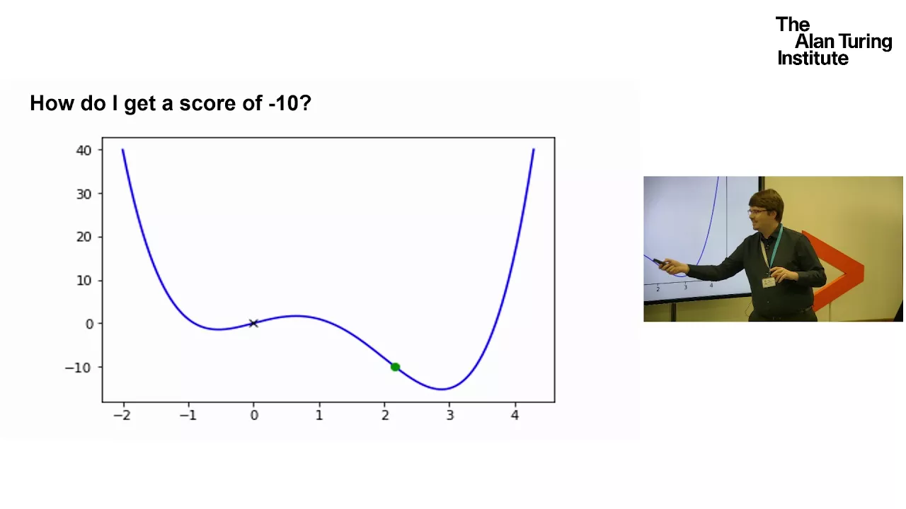
Counterfactual explanations provide meaningful transparency in algorithmic decision-making by revealing what specific changes to input variables would have resulted in a different outcome, enabling data subjects to understand, challenge, and potentially alter future decisions; unlike traditional model explanations, this approach decouples explanation complexity from classifier complexity, works with any algorithm including black-box models, and is grounded in psychological research on how humans naturally seek contrastive explanations to understand causality and make informed decisions.

AI models exist on a spectrum of interpretability: white box models (decision trees, linear regression) are fully interpretable, while black box models (deep neural networks with billions of parameters) are nearly impossible to understand. More powerful models that handle complex tasks tend to be less interpretable. Explanation techniques include: local explanations (SHAP values) explain why a model made a specific decision for one individual; global explanations (feature importance) show which variables matter most across the entire population; partial dependence analysis shows how predictions change as variables change; subpopulation analysis tests whether models perform equally well across different groups. Comprehensive bias analysis requires multiple complementary approaches: partial dependence analysis reveals whether models are biased against certain groups; proxy variable detection reveals indirect encoding of protected attributes; individual-level analysis examines how changing single variables affects specific predictions. Bias correction is an iterative process requiring collaboration between data scientists and domain experts: identify biases, discuss with experts to determine acceptability, add missing data fields or modify features, retrain the model, and repeat. The EU AI Act (expected 2023-2024) will require AI systems in high-risk applications to undergo rigorous validation including explainability analysis, data quality assessment, risk analysis, and ongoing monitoring plans. Organizations must maintain extensive documentation (80+ pages) to demonstrate compliance. The 'good enough' principle states that models should be deployed when sufficiently accurate and fair, not when they can be further improved. Excessive optimization (the 'cagoule syndrome') can introduce new biases and waste resources.

The European Union's General Data Protection Regulation (GDPR) includes a right to have a decision about you by an algorithm explained to you. This doesn't necessarily mean you get to download all the training data for the neural net and run it again with your data, but somebody has to figure out what that will mean. This represents a level of governance that is being cast into law. In many cases, it can be done quite easily, which is a good thing. This regulation addresses the need for transparency and accountability in algorithmic decision-making.
Deployment of LIME and SHAP in production environments for real-time model monitoring, debugging, and explaining model predictions to non-technical stakeholders.

Deploying SHAPash in production requires transitioning from SmartExplainer to SmartPredictor mode using to_smart_predictor(). Save predictor objects in pickle format for deployment. In production, load saved predictors, provide new input data via input() method, and use detailed_contribution() to analyze feature impacts on new predictions. This enables continuous monitoring of feature importance over time, helping identify features needing removal or addition, detecting data drift, and preparing better data for future scenarios. Explainable AI in production ensures models remain interpretable as data and business contexts evolve.

This section covers advanced analytics capabilities including model explainability, deployment, and continuous monitoring. Model explainability features help stakeholders understand predictions through feature importance plots showing which variables most influence outcomes (due date, invoice date, disputed status). Classification tables provide accuracy metrics. What-if analysis allows stakeholders to experiment with different scenarios and see predicted outcomes, making models interpretable for non-technical users. Advanced capabilities include time series forecasting for projecting monthly invoice amounts. Model monitoring ensures deployed models remain effective through continuous tracking of three types of drift: data drift (changes in input data distribution), prediction drift (changes in model outputs), and performance drift (changes in model accuracy). Deployment options include batch scoring for periodic predictions and API deployment for real-time scoring. These capabilities ensure models maintain predictive power as business conditions evolve.

SHAP provides multiple visualization tools for understanding model behavior: waterfall plots show feature contributions for individual predictions, force plots display prediction breakdowns, mean SHAP plots show average feature importance, swarm plots reveal SHAP value distributions, and dependence plots expose feature interactions. SHAP enables effective debugging by allowing close examination of incorrect predictions to identify problematic features. A key application involves identifying when models rely on spurious correlations—for example, an autonomous vehicle model that used background pixels for predictions failed when deployed in new locations with different backgrounds. SHAP helped diagnose this issue by revealing the model's unexpected feature dependencies.

For production models, Snowflake enables comprehensive monitoring and explainability. Model monitors track performance, accuracy, and drift metrics with custom thresholds and alerting capabilities. ML explainability computes SHAP values for debugging model degradation. The online feature store enables real-time feature serving for live use cases, automatically synchronizing with offline pipelines and providing high throughput without infrastructure management. This enables real-time applications like live call quality monitoring where agents receive immediate feedback on call quality, stress levels, and sentiment to improve customer interactions.

LIME generates local explanations by fitting linear models to local data samples around prediction points, working with any model type but failing to consider interactions. SHAP values provide theoretically grounded explanations rooted in game theory, assigning each feature contribution based on its marginal impact across all possible coalitions. While LIME offers model-agnostic flexibility, SHAP provides stronger theoretical support and more accurate reason codes, particularly for tree-based models. Both techniques face deployment challenges in real-time production systems, requiring careful consideration of trade-offs between flexibility, accuracy, and computational efficiency.
Interpretability Intro
4:01- 1
Explains why model interpretability is crucial for trust and debugging.
- 2
Highlights risks of black-box models using real-world examples of bias.
The Fallacy of Post-Hoc Explanations (Inherently Interpretable Models)
While LIME and SHAP are widely used to explain complex 'black-box' models, prominent researchers argue that post-hoc explanations are fundamentally flawed, especially for high-stakes decisions. First, these methods only approximate the model's behavior, meaning the explanations themselves can be inaccurate, highly unstable, or easily manipulated. Second, they can create a false sense of security by masking biased underlying logic. This counter-perspective advocates for using 'inherently interpretable' models—such as decision trees, rule lists, or generalized additive models—from the start, eliminating the need for unreliable approximations.
Up Next

Text Preprocessing for NLP: Tokenization, Stemming & Lemmatization
@activelearning4386
642 views•2022-12-10

Secure Multiparty Computation (MPC): Foundations & Challenges
@SimonsInstitute
7.3K views•2015-05-28

Neural Networks for Recommender Systems (PyData 2017)
@PyDataTV
21.1K views•2017-04-25

Neural Networks Explained: Math, Layers, and Learning Fundamentals
@3blue1brown
21.9M views•2017-10-05
Related Study Plans & Knowledge Roadmaps
Structured learning paths in Artificial Intelligence