



![[도올김용옥] 수학을 배우다, AI(인공지능) 이해를 위한 최소한의 수학 02 - 먹고살기 위한 수학? [남호성교수]](https://i.ytimg.com/vi/DH40nWuNr00/maxresdefault.jpg)








![[CW Paper-Club] Fooling LIME and SHAP: Adversarial Attacks on Post hoc Explanation Methods](https://i.ytimg.com/vi_webp/5aig2Kh9smU/maxresdefault.webp)


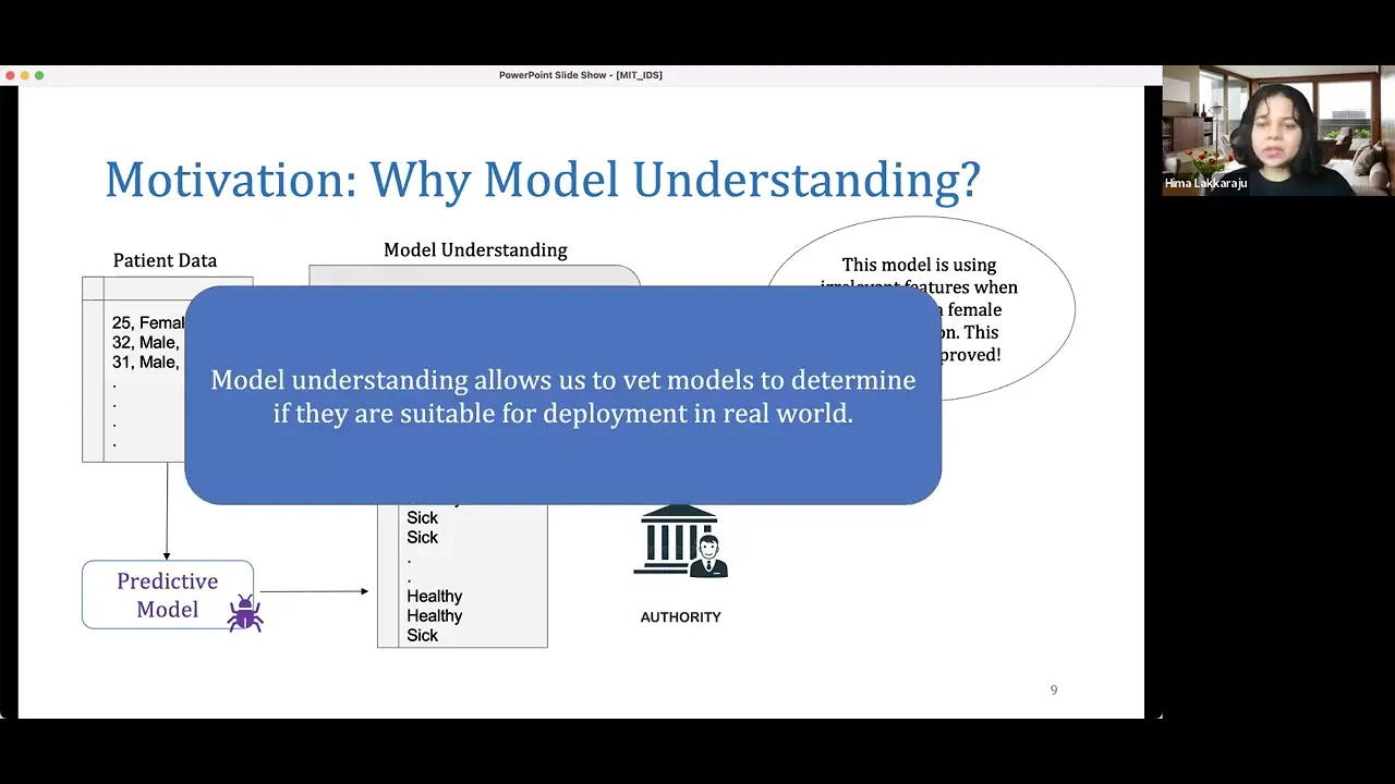


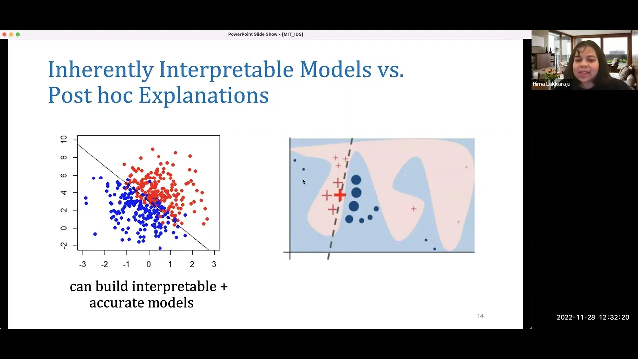
Post-hoc explanation methods provide interpretable descriptions of complex black-box machine learning models by analyzing their behavior without modifying the underlying model architecture; these methods are categorized into local explanations (which explain individual predictions through techniques like LIME, SHAP, saliency maps, anchors, prototypes, and counterfactuals) and global explanations (which summarize overall model behavior through collections of local explanations, representation-based approaches, model distillation, and summaries of counterfactuals), with the choice of method depending on the specific application context and end-user requirements.
Explainable AI: Post Hoc Methods for Model Interpretability
Added:Core understanding of supervised machine learning algorithms, specifically the distinction between inherently interpretable models (e.g., decision trees) and 'black-box' models (e.g., deep neural networks, ensemble methods).
Familiarity with how features (input variables) are represented, transformed, and mapped to target predictions in high-dimensional data spaces.
Basic knowledge of neural network mechanics, including activation functions, loss gradients, and backpropagation, which are essential for understanding gradient-based saliency maps.
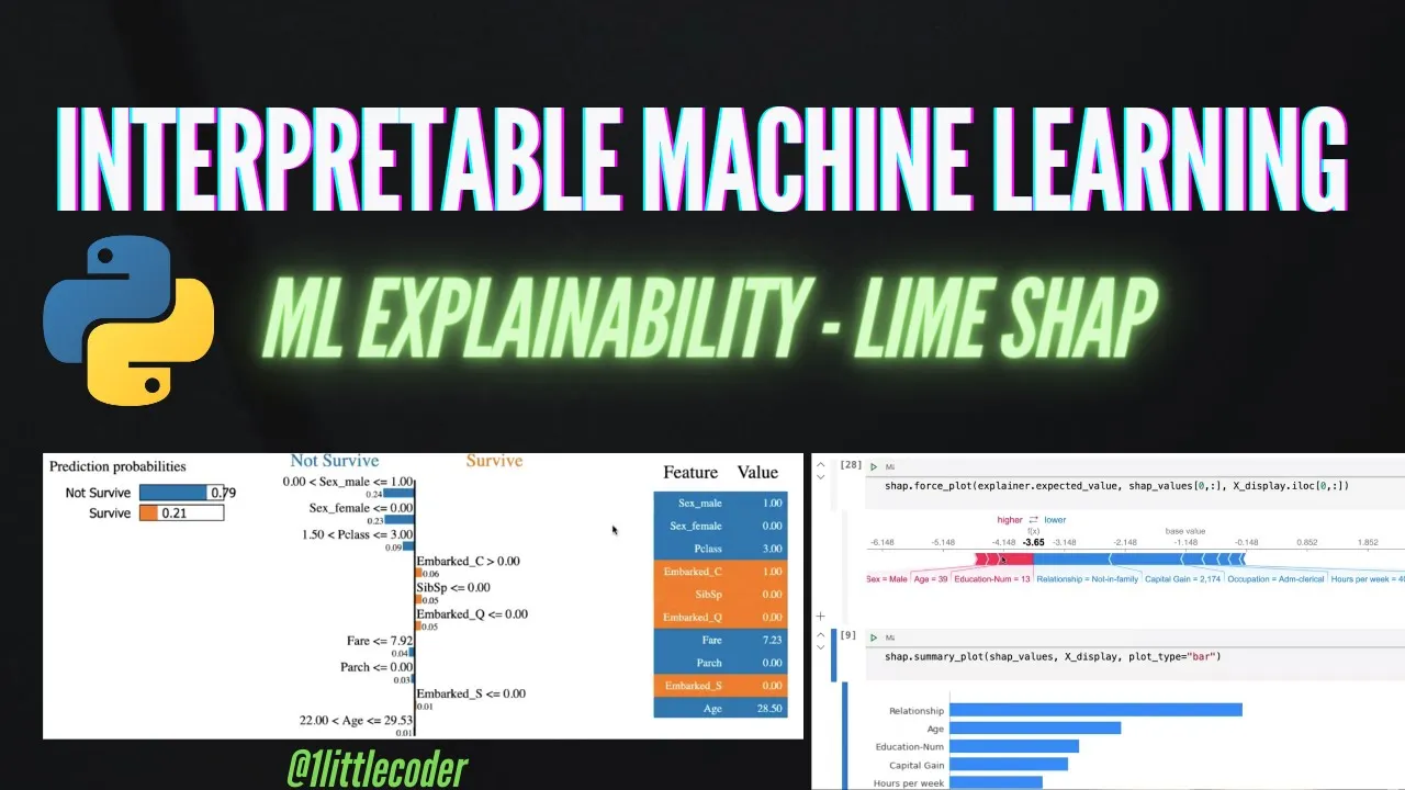
In-depth study and hands-on implementation of state-of-the-art model-agnostic frameworks, specifically LIME (Local Interpretable Model-agnostic Explanations) and SHAP (SHapley Additive exPlanations).
Methods for quantitatively evaluating the faithfulness, robustness, and stability of post hoc explanations to ensure they accurately represent the model's true decision boundary.
Exploring adversarial attacks on explainability methods, focusing on how black-box models can be manipulated or 'scaffolded' to yield deceptive explanations.
Applying counterfactual explanations to algorithmic recourse in highly regulated industries, such as automated credit lending, insurance, and healthcare.
16.5K views212likes1:12:37Original Release: 2022-11-04
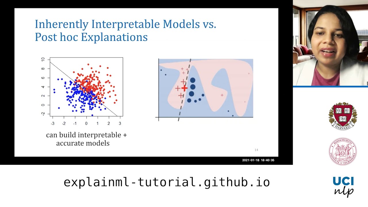
all right let's get started okay okay so part two of our discussion so now we're going to focus on post hoc explanation methods right so let's think about explanations a bit more because unlike what we have been talking about so far uh there is no longer a model that is trying to be inherently interpretable here or produce things that can be interpreted right so now we are in a situation where we essentially have this kind of a complex classifier we can't touch the classifier or that's the setting that we are working with we don't want to change anything about this classifier but there's an end user and we need to sort of provide some interpretable description of this model's Behavior to the end user right so the explanation will be an interface between this complex model and the end user so it has to almost have two Key Properties so the first thing is the explanation should Faithfully describe the behavior of this classifier right so if the explanation is not correctly describing Model Behavior then essentially it's not useful even if it is interpretable to the user right that's one piece of it and the other side of it is whatever we are producing should be able to be should be interpretable to the end user right so those are the two pieces and then the sort of complexity in this entire scenario comes from what exactly do we mean by understandable to the end user and that depends quite a bit on the nature of the end user themselves right so whether they are machine learning experts whether they're domain experts all of those aspects and you know that's something that we are going to also talk about a bit more later all right so for example when we think of oh we just need to provide an interpretable description of the Model Behavior that could look like any of the following for example you could just send all the model parameters Theta and if this is somebody who is building a model themselves or you know is a scientist research or engineer who under understands machine learning they may be able to make some sense of it right so that's some form of like providing that person more information or you could basically send many example predictions and say that you know for this example this is the output I get for such examples is the output I get and so on or you could summarize with a program or rule or a tree all these kinds of constructs that we talked about earlier or you could sort of Select most important features or points that are influencing the prediction or you could sort of describe how to flip a given model's prediction so all of these are possible explanations of a complex model to an end user right now which one is more apt depends on exactly what your application is and also who your end user is right so for example I can't send all the model parameters Theta to a doctor and assume that they would make any sense of it right but whereas if I tell them things like most important features they might be able to use that information okay so very high level the literature on post-talk explanation methods can be divided into two classes of explanations so one is local explanations and the other is global explanations I think the names are pretty descriptive but like let's just walk over what these means right so local explanations the goal of these these explanations are these methods is to explain individual predictions of the model right so if we have one prediction how is that prediction coming about or what are the factors that are impacting that prediction now global explanations on the other hand they try to describe to the most part complete behavior of the model so they try to give a global picture of the model's Behavior okay so their goals are also slightly different again you know because of the way they are sort of like thought about uh local explanations typically help us unearth any kinds of biases or models Reliance on spurious features Etc in a given local neighborhood of an instance whereas Global explanations help shed light on Big Picture issues or big picture biases affecting larger subgroups in the population right and uh again I guess it kind of follows from what we are discussing earlier so by local explanations help vet if individual predictions are being made for the right reasons uh Global explanations help with if a model at a high level is suitable for deployment right so these might seem like somewhat trivial issues but like in practice these things are important because for example before we even deploy a model so there needs to be let's say in a hospital or you know in a court system and so on there needs to be like approvals or high-level authorities need to approve that okay these models are you know fine enough to be deployed right so for in that case we can't give them you know a bunch of local predictions of like 1 million points and say now use this to wet your model so for them the global description is very important so that they can see a big picture view of what's going on right so in practice these differences play a very significant control in enabling certain applications and practices versus the others okay all right so this is broadly the needed to look at so first we are going to focus on local explanation methods under that you know the thing about you know sort of what we discussed so far and how it ties to this is you might see some familiar constructs here that we already talked about in the context of inherently interpretable models right whether it is the rules whether it is you know feature importances whether it is prototypes these constructs will be repeatedly occur through this entire literature whether you're talking about inherently interpretable models or Post drug explanations okay but these bring a whole new set of challenges with them because you know we are considering approximations of another model here right okay so let's jump into the first and a very popular class of local explanations which is feature importances right uh so I'm sure some of you have heard of this method called lime or shap you know because these are pretty popular and if you're looking for I want an explanation method you might run into repositories and you know packages which have implementations for these right so this this was I think one of the initial methods that came up within this area of post-hoc explanation methods and the algorithm or the actual method is actually very simple and intuitive right so what this is trying to do again remember that there's a local explanation which means we are trying to explain individual predictions of model just one prediction at a time right and the way this method works is let's say our goal is to sort of explain the prediction of the model on that instance that you see on the screen and the models the underlying models decision surface is this kind of complex non-linear surface that you see uh you know sort of below the plus Mark and the way you sort of proceed with this algorithm is that you take that point let's call it x i and then you perturb that point several times and you basically generate instances around x i right so you add some random gaussian noise to X and then you generate a bunch of instances in the local neighborhood of X or x i all right so now use the underlying model to predict the labels for each of these perturbations that you generated right so now take the underlying model and determine the predictions of each of those points and then uh weigh these samples according to the distance to x i right so points that are closer to X I will get higher weightage and points that are farther away from X I will get lower weightage and essentially you do that waiting and then you basically fit a simple linear model like a linear regression or a logistic regression on these weighted samples okay so that's pretty much what this does and now your simple linear model it gives you a bunch of coefficients or weights associated with different features and that becomes your explanation because that provides feature importances okay so the algorithm is super simple as you can see so you literally take a point put up it a bunch of times generate a local neighborhood and get the model's predictions on that local neighborhood and then fit a linear model on those instances and their predictions right so that's it okay all right so uh this paper also kind of gives some interesting examples which have become like classic examples of thinking about explanations and their necessity and we have already seen some of this in our motivation for example if we just look at the predictions made by let's say some models we might see that oh there's only one mistake so maybe the model is actually doing extremely well right so it's predicting everything correctly there's only one image where it's making a mistake but on the other hand once you see the explanations output by this method what you realize is what we have essentially built is a snow detector right so this kind of insight can only be obtained from uh explanations okay so uh alongside lime another popular method that often comes up when you think of or when you actually even search for post talk explanation methods is called shap right so shap is also trying to play along the similar intuitions as that of lying and it has a lot of connections with lime but at a very high level what shap is trying to do is estimate marginal contribution of each feature towards the prediction and you sort of average this contribution across all possible permutations so what I mean by that is let's take an example where we have uh three features so X1 X2 and X3 okay and now we want to come up with this feature importance according to shapley values for X1 right so we want to determine what is the contribution of X1 so the way shop operates is actually very simple but you know scalability issues arise which which needs a lot more tricks to happen in the background for that to work out but essentially the idea is you compute how much does the prediction change prediction of the underlying model change with or without X1 for different permutations of the features right so first you see okay so with no features what will be the prediction if you add X1 what will be the prediction okay then with X2 alone what will be the prediction if you add X1 what will be the prediction what's the difference and again the marginal contribution of adding X1 to X3 right so essentially for each such combination you are Computing what is the result of for example adding X1 to the mix minus what is the result of not having X1 in the mix right so you do this for every possible future permutation and then you sum up and average all those marginal contributions so that's what will constitute the shapley value or the contribution or importance of each feature and this is how you can compute it but as you can see you know once you get into permutations a lot you know this will become a very hard problem to solve computationally and there are tricks for approximating these and so on but you know that we are not going to get into but here is the high level intuition okay all right now in this class also there are some rule-based methods which are pretty popular so one of them is anchors which can be thought of as a rule-based variant of line we talked about right and anchors essentially relies on the same tactics as that of line so what we do is if you want to uh sort of think about the explanation of an instance X you perturb that instance X to generate the local neighborhood just like you did for lime and then what you do is you try to find a rule that sort of correctly covers that local neighborhood right so again if you recap and think back to this decision sets or rule sets that we were talking about there also the goal was to find some rules which nicely and correctly cover a certain space or the data set in that case here we are just trying to find the rules uh that correctly cover the local neighborhood so the intuitions are the same uh we're not going to go over the details of the algorithm but roughly you are trying to find rules that cover the local neighborhood correctly so for example let's say here is a data point and this is the prediction of that data point uh so lime's explanation will basically tell you the importance and the direction of the importance positive or negative for each feature whereas anchor explanation is basically that rule that is sort of covering the local neighborhood okay okay so the next class of local explanation methods that's very popular especially in images and computer vision is sale in cmaps and saliency Maps again these are also going to Output some kind of feature importances but they sort of do it in a very different way than alignment shop let's take a look at those okay so with saliency maps the idea is that let's say you have this complex model and you know you can input images to that model and then it basically makes predictions in this case the model is saying the image is that of a junko bird the question that you're asking is what parts of this image are most relevant for the prediction junko bird right so that that's the question that you're asking and you're hoping to get an output like this which basically highlights the important pieces within the image that the model is relying on when making that prediction junco bird okay all right okay so uh just for the sake of I think thinking about different classes in this settings so either you could think of a binary class model or a binary classifier where there's a function f mapping you know to class one or if you have multiple classes you can think of a class specific logic right and F5 is a class specific Logic for class I okay so there are several methods in order to generate these saliency maps that we just saw and a lot of these basically play on gradients rights or derivatives to put it more simply so for example the first method which actually uh was popular for a while before of course then peoples are detecting issues with it and so on is this input gradient uh where what you are trying to compute is basically the gradient of that class specific logit right so gradient of that function or the underlying model f of x with respect to the instance X whose prediction you want to explain so what is the reason behind doing this it's a very simple intuition right so you want to see how much does the output change or how much does the underlying function change when you make a small change to the given input data point right or each of the features of that input data point essentially right if y changes a lot as a result of changing one particular feature in your input points Vector then essentially that feature is very important for y right so that's it you know rate of change of Y given X that's essentially the principle you are using and you are Computing this and you know things that have higher gradient values here will basically mean that the features are more important okay all right so uh if we sort of take this example and visualize the heat map where red indicates the regions of higher importance and white is regions of less important here is a kind of outputs that were produced by these input gradient methods right and you know several challenges exist with something like this first of all this is visually noisy and somewhat difficult to interpret and there are also other issues such as gradient saturation that have been like documented but mainly if you look at this image you know we can see that it's somewhat noisy we are not sure what to make of it what is the model looking at is that what the model looking at and so on so in order to fix some of the issues with these methods there was a variant proposed called Smooth grad and what smooth grad does is essentially it averages the gradients of noise the input it does not just take X and compute the gradient of the function with respect to X it basically takes X perturbs it n times and then computes the gradient of the output function with respect to each of these perturbations right and then you average all that so you are essentially creating a smoothing effect in this case when Computing the gradient right and so this is the output for the same image with smooth grid as you can see there is you know you can make a bit more sort of sense out of this it is not as noisy as what we were seeing with gradients right okay so the next approach that was proposed again along these lines was that of integrated gradients and the idea here is again you're trying to sort of do some smoothing of the gradients here but a slightly different kind of smoothing than averaging the gradients right so the idea that's being used here is do a path integral which is basically compute a sum of the interpolated gradients so you'll think of this as there is some baseline input X tilde you can think of that as like just a black image right with nothing on it so there is some baseline input and the way you are thinking about gradients here is you are interpolating gradients between the Baseline input and the point okay so you're basically going through all the gradients in between and trying to compute the integral of all those gradients on that interpolation okay and you know again the output started becoming more and more clearer as people improved these methods one on top of the other and there are also a few other methods for example there is gradient times input which is you don't just compute the gradient you also do a DOT product with the point x itself so that's the element wise product of you know gradients and the input points uh so that is what produces like images like these uh and there are more variants for example there is lrp layer wise relevance propagation grad Cam and so on but the point of these kinds of methods is they use gradients in some way or the other and create like you know different versions of smoothing of these gradients to sort of come up with the saliency map or the explanation and this is a pretty popular class of post talk explanation methods that are commonly being used in a variety of applications including Healthcare like for example using chest chest x-rays to sort of detect tumors and so on people are also using these kinds of methods for generating explanations there okay so the next class is prototypes and example based post-hoc explanations so under this broad area again there are several approaches so there's just probably a running note for everything so I think we are touching some representative approaches in each class or each category there are several other approaches that you know due to time constraints we are not able to get into but the goal is to give you a high level idea about each class right okay so with the prototypes or example based explanations there are two key methods that have been proposed under this category at a high level these class of methods use examples whether they're synthetic examples or natural examples to explain individual predictions right so the first work is by priscilliang and his student pangwei which is on influence functions the goal here is to basically identify instances in the training set that are responsible for the prediction of a given test instance right so if you have a test instance which of the K training instances were responsible for this prediction that's what you want to identify and the second is called active activation maximization where the goal is to identify again examples whether synthetic or natural that strongly activate a specific function of Interest or a neuron of Interest okay so let's talk about the first approach a little bit and then go to the second one uh so here as I was just explaining this is the first approach what we want to ask here is not just look at what pieces of the image are influential to the prediction but ask the question of which training points have the most influence on the test class for this particular point and the prediction right so for example in this case you know the answer might be some other images in the data set that are of a junko bird right and the approach or the technique that is that was used in this work is actually borrowed from a very classic technique in robber statistics which is titled influence functions and the goal of while while in the classic statistics literature that this was obviously not used for quote-unquote explanations uh there's something called as Cooks distance in uh you know classic lobus statistics literature the goal here is we are trying to estimate the influence of each of the points in the training data set on the model parameters right so in order to do that for example if I want to estimate the influence of this point on the model parameters one way is you know I remove the point out train the model again see how the model changes right but that quickly becomes complicated if I have to do it for every point so there is an uh there is a very popular measure called as Cooks distance which actually gives an analytical expression for computing the change in the model parameters when you sort of like remove a point from the data so essentially you're Computing the influence of that point right so what this paper does is essentially take that basic idea of Cook's distance and apply it to a modern machine learning setting of thinking about explanations and influence of training points on test points and so on right so for example let's say x j is basically a training sample Point uh sorry Z J is a training sample Point z i is basically indicating any point I in the data set and there's also some test Point Z test okay so for those of you who are familiar with machine learning this is like a classic empirical risk minimization sort of objective function and this is what we used to learn model parameters right so these approaches they sort of think about this slightly differently in the form of an updated ERM solution so let's say our goal is to estimate the influence of the point Z J on the model then you can sort of think about that kind of an updated solution and if you set Epsilon to minus 1 by n that is effectively like you know sort of removing the point Z J from the data set okay so this is a slightly generalized formulation so that you can think about the influence of the point Z J on model parameters so basically they use that to sort of compute uh this kind of influent influence of the training points on the model parameters right so that that's the main goal so ultimately you want to get to this where you want to compute the influence of a training Point Z J on the model parameters and as you can see that involves Computing a Hessian and once you have that then you can estimate the impact of ZJ on the loss of Z test which is a test data point by using that expression okay and this paper also talked about a bunch of explanations here one is you can sort of compute self-influence of a mislabeled examples to understand what is happening right so if a point is misclassified if we compute the influence of that point on the predictor then we can see or potentially understand why that misclassification is happening or we could potentially diagnose like a possible domain mismatch where a point is out of distribution and you know we can sort of see that by looking at the training examples that are influencing the prediction of this point and also because this is helping us identify influential points in the data potentially if we poison or if adversaries poison those points then they may be able to change the predictor maximally right so there are several sort of like other applications uh boiling down into adversarial examples and other kinds of literatures of this approach so there are a couple of challenges with this kind of approach though so one is scalability because it involves Computing a Hessian as we just saw right so that can be hard in practice uh and the non-convexity of the objective we are looking at that also turns out to be challenging in practice and there are some other papers that try to fix some of these issues okay the other approach that we considered under this setting is activation maximization so this approach again the goal is to identify examples that activate a neuron of Interest right so and then you know the different implementation flavors here are so one is search for natural examples within a specified data set a trained data or so that strongly activate a neuron of Interest or synthesize examples that may not necessarily exist in the original training data typically why optimization procedures like gradient descent that strongly activate a neuron of Interest right so either use optimization to find synthetic examples or search in your data set to find the example so here are some examples that were sort of like output by using each of these approaches the top row is basically examples chosen from the data set itself right so which were activating certain neurons in a particular intermediate layer strongly and the bottom is if we use optimization to find such examples what they look like so clearly there is a big difference between the kinds of examples you see in both cases right so in some sense the top you can sort of see it's showing some baseball images or you know stripes and then the bottom is like it's a clear sort of like ambiguity there that whether it's a baseball or Stripes is unclear so the images that you would get when you think about natural examples versus synthetic can look quite different okay right okay so now the last class of local explanation approaches is counterfactures which actually has been popular because of other kinds of applications than the ones that we have been talking about right so at a very bare minimum level what is a counter factual explanation counterfactual explanations tell us what features need to be changed and by how much to flip a model's prediction right so for example in this case what features in this image of a crested are need to be changed and to what uh in order to get a red face camera right so why is this important or like where is this useful this is an interesting question because a lot of this area of research is thinking about applications in banking and financing uh because as I was saying earlier like regulations like gdpr are sort of focusing on those areas as their preliminary areas of enforcement so this these explanations have become popular because of those areas so just to understand a scenario here let's take a look at this example where there is a loan applicant who has submitted their loan application to a bank which has a predictive model which determines if that person should get a loan or not right so in this case if the person is denied a loan instead of just saying that the person might actually benefit if we tell them what they need to do in order to change their profile and reapply for a loan so that they have more success next time they reapply for a loan right so now how do we generate such explanations is basically this area of counterfactual explanations also referred to as algorithmic recourse so these terms are often used pretty interchangeably in the literature today so whenever you hear one or the other you're basically referring to the same thing right and the recourse or the counterfactual explanation takes a form of something like this feature and then the change to the feature right so for example salary increase salary by 5K you know pay credit card bills on time for next three months so that's the kind of changes that are recommended using these algorithms okay so the strategies for generating these kinds of uh explanations are many but they have some common underlying principles so I'm going to touch upon those first before I get into other details okay so generating counterfactual explanations at an intuitive level you can think of it in a very simple way right so your goal is there is some point x on this negative labeled area of the model decision boundary and you want to find another Point uh in the positively labeled area of the decision boundary that X can morph into right so that's the problem so intuitively you can think of it as so now take the point x and keep perturbing it and pushing it towards the decision boundary and once it crosses the decision boundary stop and say x should become that point in order to get a loan right now the the question here though is if I take X and start perturbing it towards destined boundary it can either go this way and become this point cf2 or it can go this way and become this point c f 1. which should it become right so that is basically where different approaches differ on so in some sense the proposed algorithms for solving this problem differ on how to choose among these candidate counter factuals and the second thing is how much access is needed to the underlying predictive model okay whether they can work with a black box or whether they need access to the gradients of the underlying model right okay so we'll get into some of the details of these approaches now and just go in sequence to see how they sort of go from one to the other uh or actually let me pause here and see if there are any questions before I do that and go into more details there is there is one question from the uh chat here that might be relevant to what we were talking about just previously um and the question is generally what do you think of anthropic's recent softmax linear units paper um does it give more hope for building more interpretable model architectures or should we be focusing on these post-hoc explanations that you've been talking about yeah I mean I I would say all the efforts uh you know whether you're trying to sort of do it at the level of the model whether you're making models more smoother right or whether you're using post-doc explanations these are all efforts in the direction of making something more understandable in some way or the other right so at least in my personal opinion the answer is probably not one versus the other uh but I think you know sort of having a more clearer characterization of when to go to that and when you know would that fail and in that case would something else help So currently and we'll talk about this a bit more as we go towards the end of this I think all these approaches are useful it's just that I feel what is needed is a clearer understanding instead of saying it's a this versus that battle a clearer understanding of here is when this would be more useful and here is when something else might be more useful I think that's where we should be headed because this is something that I get asked a lot in different forums as to also like you know maybe we should never use post-hoc explanations because there are some disadvantages which we'll talk about at length uh in the afternoon session uh but I think the answer is probably not to pick a side but like to see when each approach would be useful okay all right um so let's move forward and try to look at each of the individual approaches in this area so here is basically the core objective of like a lot of approaches that try to generate counterfactual explanations so the idea is given a point x we want to find a point x Prime such that the distance between x and x Prime is as small as possible and the model's output on X Prime is a positive label right so you want to find the closest instance to the original instance you started with such that you know these two are pretty close but also the label of this new instance that you're finding is a positive label right and then you ask X to change into X Prime basically that's the idea okay so X Prime is called your counter factual and X is your original instance and D can be some distance metric whether it's l 2 distance or you know some other kinds of distance Manhattan distance and so on okay uh so the choice of distance metric is also important because if you're thinking about a practical application this can dictate what kinds of counterfactuals are chosen right of course in terms of your optimization methods and stuff you know it might make some difference but I think there's more of something that would make a big difference in practice okay so the first paper that actually touches upon this area is uh presented by Sandra wachter and her colleagues and they use normalized Manhattan distance here but you know other papers which build on it have started using L2 as a classic distance metric because it improves the optimization pieces okay so now uh so that that's basically your minimum distance counterfactions right so this is the objective typically when solving this objective walkthrough and even other methods in this area essentially try to make this constrained optimization problem as an unconstrained one by bringing up these constraints into the objective itself and then they basically you know solve this differentiable and constrained version using optimization algorithms like Adam with random restarts right so as you can see there's already a non-convex problem so you would need random restarts in order to uh have a chance at getting to the global minimum all right so this particular method actually requires access to gradients of the underlying predictive model so the predictive model can't be a total Black Box where you're just seeing the predictions of the model you need to be able to compute the gradients of the model right so here are some examples that this method produces so for example it says you know if your LSAT score was 34 you would have some predicted score of zero and you know if you change your LSAT score to some value then this is what would be your predict predicted score right so the interesting thing is just the way this method is implemented it's suggesting people to change their race in order to get a desired outcome right so obviously something like this is not feasible to act upon in practice but also it is highly unethical to sort of do these kinds of things right so that's why there are further approaches with sort of built upon this approach and that's the work by usted netal where they change this objective to now uh enforce that X Prime which is the counterfactual that we are picking should belong to a particular set a which can be be thought of as a set of valid counterfactions right so in that set a for example you will not allow changes to raise or gender or any other sensitive attributes uh that are you know unethical to use okay okay yeah all right so here as I was just talking about this is a set of feasible counterfactions that is often given by the end user and changes to race and gender and these kinds of things are not feasible right and there is also an additional thing that you see there that has changed from our first objective that we considered which is instead of distance this approach is now considering costs so in some sense instead of just saying I'll compute an L2 distance in this sort of data space it's saying you know some features might be harder to change for a person in practice than others right so let's try and account for them like maybe for somebody who is living in a particular place it is easy to increase the size of their house or the square footage of their house but not their salary and for somebody in another place the vice versa could be true how can we incorporate those better when recommending these changes so let's not just look at the distance in the input space but look at the cost associated with changing certain features when prescribing this kind of a recourse right and as a first sort of a cut you know solution to this this particular approach sort of models cost as a log percentile shift which basically models this aspect that changes become harder when you are trying to make changes at like higher percentile shift right so changing from 90 to 95 might be much harder than going from 50 to 55 percentile for example okay so this of course what this approach does several follow-up Works including some of ours actually try to learn these costs by asking users about their preferences so for example we did some work where we basically go and ask users people are bad at assigning this cost straight up to a feature but if I tell them would it be easier for you to change your salary versus the square footage of your house they can give a yes or no answer and do pairwise comparisons well right so how to go from there to inferring such costs is of course some follow-up work to this that we and other researchers have done yeah okay so basically this approach or this paper only considers the case where the model is a linear classifier so that's and they also have theories surrounding this in order to say that whatever you're getting out of this is a good solution for a linear classifier so the way they solve this problem is they formulate it as an integer program and optimize it using cplex so this approach actually requires complete access to the linear classifier they need the weight Vector in order to compute this kind of a recourse or a count of actual explanation right so which may or may not be available depending on the setting you're working with okay all right so now the question is what if we have a black box or a non-linear classifier uh instead of a linear classifier now one potential solution could be something like you know generate a local linear model approximation for example using an approach like line that we talked about earlier and then once you get such a local linear model then apply you know this framework in order to get the recourse that's one approach it of course has its flaws and Depends heavily on the quality of that local linear model approximation itself but you know that's the sort of potential way to use this approach with a non-linear classifier right and this is an example of how the output from this particular approach looks like so basically it has some features to change and what's the current value and what are the required values so essentially that's the kind of output that these approaches give right uh so now here like let's say there is this value called as current depth and you want to decrease that but one more piece to notice is that in reality in practice changing one feature without affecting the other might not always be possible right so what do I mean by that for example we just told this applicant reduce your current depth from you know 3000 to 50 to 000 and let's say after one year this applicant comes back and say oh my current debt has reduced to thousand Now give me a loan and then the model might say oh but your age also increased by one and this recourse is no longer valid for people whose age has increased by one along with your depth reducing right so now you know it's very important to account for for these feature interactions when generating counter factuals but how do we do it is basically the next practical problem which was addressed by some works right and the solution is kind of what you might be expecting by now which is you play with the set a which is basically the set of feasible counter factuals that you allow when trying to pick a particular count of actual for a person right and in this case you will now sort of resort to using structural causal models so for example let's say you have access to the causal process that is generating the data which captures all the interactions between different variables in the data and how they interact you can use that model and allow only those changes which are permitted according to that causal model right so that's one approach which was suggested in in literature but the big question is what if we just don't have access to the structural causal model which is often in the case because with any real world data set you really get access to a full-fledged causal model of the underlying generation process there are also sort of other works which try to work around this problem one approach basically tries to say if you have imperfect causal knowledge like you kind of know some relationships you will try to infer the others and then leverage that or the more recent approaches that have become popular are based on variation Auto encoders so the idea is ultimately you want a realistic enough counterfactual right so that's your goal with all this even when you look at structural constraints and so on you're saying my counter factual should not look unrealistic so how do I generate more realistic counterfactures whether it is using the causal graphs or whether it is using some other approach right and the other strategy or an alternative strategy that was sort of considered or you know is becoming more popular these days is so the goal is the generated counterfactuals should lie on the data manifold so the approach taken is construct variation Auto encoders to map input instances us to a latent space right and then you search for counter factuals in that latent space and once a counter factual is found map it back to the input space using a decoder okay so this basically helps with a bunch of things including the fact that your input feature space may not always be smooth or continuous whereas the chance of your latent piece being that is higher so you're likely to use a gradient descent and get to a point uh that you want to give as a counter factual uh more nicely in your latent space than you might be able to do so in your input space partly because input space could also be discrete and you could have features that are just binary valued or like rank ordered and so on right so that's that's what this approach is trying to tackle okay so with that we are pretty much at the end of our local explanation approaches module and again between these two approaches local explanation approaches have gained a lot of popularity compared to even Global explanations in the literature and also in terms of adoption okay so before I get into Global explanations and go over some of the approaches there I'll pause here briefly to see if there are any further questions about local post-hoc explanations yeah so you you go back by basically using the decoder so when you develop the encoder and decoder so decoder will map this point back to the input space and that will help you generate like realistic enough points in the input space correlations with good teachers everybody goes with because of advances correlation maybe I don't know it's safe male pregnant you might get this type of strange right so the hope is that I think because this approach does not add anything more on top of you know the decoder to ensure some of these things I think the hope is that when you do this encoding decoding process or especially the encoding process you're preserving some of these kinds of relationships in the data because they may appear prominently but as of now this approach does not add anything else to the decoder so if something gets missed in terms of like how the encoder is capturing these relationships you might still run into those problems but the hope is that that will be taken care of by the encoding yep okay all right uh okay so let's go to Global explanations and the goal here kind of contrasting from what we were saying so far uh is to explain the complete behavior of a given Black Box model right so in some sense we want to provide a bird's eye view of the Model Behavior and you know the why do we need this is it can help us detect the big picture biases persistent across larger subgroups for example the biases persistent against let's say a minority group or a particular gender or race you can sort of see those better with this kind of a bird's eye view right that's the goal um and well one might think well I have local explanations I know how to compute them why can't we just inspect these local explanations and then learn about the big picture Behavior as we can already see intuitively that's very hard to do in practice because if you have 10 000 points manually inspecting all these local explanations and trying to make sense of them is going to be extremely challenging from a cognitive overload perspective for people right so that's why we want a better summary of the local explanations and that's what Global explanations are trying to do okay so in some sense Global explanations are complementary to local explanations in terms of the view they take on the Model Behavior okay so we already talked a little bit about some of this so I'm not going to go over that again instead let's look at some of the categories of global explanations so people have again thought about different uh you know approaches to sort of generating Global explanations so one is think of them as a collection of Representative local explanations uh so we'll discuss how to do that the other is representation based explanations which is a slightly different category than all the sets of things that we have seen so far and then there is model distillation which means you are just trying to sort of use a simpler model to approximate this existing complex model as accurately as you can given the constraints of the expressiveness of the simpler model and then you know with respect to counter factuals what can we do with global explanations so those are the different approaches that we'll touch upon okay all right um so let's think about the first approach which is global explanation is a collection of local explanations right so how to generate a global explanation of a black box model so the high level idea is generate a local explanation for every instance in the data using one of the approaches that you've discussed we have discussed earlier and pick a subset of K local explanations and then return that as a global explanation right by saying you know instances which look like this have this kind of explanation that's how you're thinking about a global explanation but I guess the key question in terms of the exact algorithms you use are well what local explanation technique to use and how to choose this subset of K local explanations right so to this end different approaches were proposed and again let's talk about this first in the context of line uh so that we can understand how to pick a subset of K local explanations right recall that lime is used to explain a single prediction so essentially if we are looking at that point that is labeled in the black color it can provide you a linear model that approximates the behavior of the underlying model in the locality of that point right again we have been discussing about this challenge of like it's hard to examine all the explanations so how do I pick K so that's the question right so these K explanations are a subset of K explanations that we pick should have two characteristics so one is they should be representative in some sense they should summarize the model's Global Behavior and the other is they should be diverse they should not be written in descriptions right so for example let's say if I have picked the point already that is labeled in black color and its Associated explanation in my Global explanation I would rather pick the blue point and its explanation next instead of the red because the red is essentially the same way linear model right given that you are trying to only pick K points and their explanation to give a global summary you don't want to pick redundant explanations right so now how do we do this essentially this can be formulated as a submodular optimization problem and a greedy approach can be employed in order to pick such explanations right so you basically start with start at some point pick an explanation and then maximally try try to pick explanations that differ maximally from this explanation that you have already picked right so that's the way in which you can intuitively think about this process and you know this approach is model agnostic which means you don't need access to gradients of the model functional forms of the model architecture of the model all you need is you should be able to throw a data point at the model query the label of the point and get it right so that's true even of lime and shap and some of these other approaches by the way that distinction often of how much access you need to the model becomes important again in practice because in certain settings you may not have access to say model gradients or model architectures or their functional forms okay all right so similarly there is another approach called SP anchor so which is essentially what we you know thought about for lime it's an analogous extension but for anchor algorithm and it produces rules right so use the anchors algorithm to obtain these local rule set for every instance and then use the same procedure to greedily select a subset of K local explanations and then return them as a global explanation okay all right so let's talk a little bit about representation based approaches because these have gained a lot of popularity in recent times but have also encountered a lot of pushback okay and you'll see why in just a bit uh so the goal of representation based approaches is that you're trying to derive model understanding by analyzing intermediate representations of a deep neural network right so in some sense your main goal in doing so is to see how much do models rely on Concepts that are semantically meaningful to humans so what we want to go from where we want to go to is so far we are saying okay you give me a bunch of input features and I'll tell you the importance of each of these input features on the prediction right but what we are saying is what if I as a human will tell you a concept that's not a feature in the data for example let's look at this scenario right so let's say we are looking at this particular prediction where you have the image of the zebra and there's a model that takes this image and predicts the label correctly right now if I want to ask the question how important is the concept of Stripes to this prediction where Stripes is not an encoded feature in the feature space I know what Stripes is as humans we know what that concept means right but the model does not for for the model it's all pixels right so it can only compute importance on the pixels in the image but now you're saying I have a concept in my mind how important is that concept to this prediction okay so how to do that is basically this area of representation based explanations okay so the one of the approaches that's popular in this area is called TCAP and the way this approach approaches this problem is as follows right so let's say now our goal is to estimate the importance of or influence of the concept called stripes on the predictions of a model okay so for this first of all I need to tell the model or tell your algorithm what Stripes even mean right so to this end I'll give my model two sets of images the top set of images that you see is all capturing the concept of stripes in different ways right and the bottom set of images are just random examples which have nothing to do with stripes so I'm giving two sets of images one from the stripes class and the other from a class that is not Stripes like a random set of images right now I pass these two sets of images through the model whose predictions I'm trying to explain and you know know let's let's pick a particular layer let's say you know the health layer which generates a bunch of representations so let's say our goal is to basically determine how does the concept of stripiness in some sense influence like the representations and the health layer of this network okay so let's say that that's the goal or you know in fact there is more we want to say about the prediction but we can literally do the approach that I'm going to discuss at each layer and then sort of you know compute the Aggregates over all the layers to determine what is the influence of the stripiness concept on the output okay but let's just pick the health layer at this point and let's take the representations generated by it that layer by the model for each of these images both the stripe images as well as the random images right and you know let's say that that's what we are basically getting at the health layer for each of these images now we build a linear classifier which basically separates these two classes of vectors so all that linear all this linear classifier does is essentially say uh for this particular image so here is the vector set or here is the vector that this would you or it is just basically trying to separate the class is this Vector belonging to uh you know the stripes class or is this Vector belonging to the random class right so that's what it is doing okay uh and then now using this sort of linear classifier that we fit we can actually compute a vector uh that is orthogonal to the decision boundary and moves in the direction of the concept of Stripes right so if you see this vector v c l it's orthogonal to the decision boundary it is pointing in the direction of the stripes class and away from the random class right so why are we doing all this exercise our goal goal is to basically get a vector representation of the concept Stripes right so if I tell Stripes to the model like you know Stripes is a concept that makes sense to me but not the model Now by doing all this I generated a vector representation in the space of the representations in the health layer that corresponds to the notion or the concept of Stripes okay so once we have such a vector then we can leverage this and compute gradients do all other things in order to get the importance of this Vector on the outcome right so that that's basically the logic that's being employed here so just to recap this whole process the goal is you'll start with two sets of images one set of images represents the notion of Stripes the other set of images represents random examples and then you get the vectors for all of those images from the model from each of of the layers actually and then you try to build in your classifiers that separate the two classes of vector activations and you take the vector that is orthogonal to the decision boundary pointing in the direction of the concept of interest and then you compute derivatives by leveraging this Vector to determine the importance of the notion of stripes on a given prediction right so the key thing here is we went from having the concept of stripes in our mind to getting a vector which quantifies what is the notion of stripe to the model right okay great so uh let's move to the next class of uh Global explanation approaches this is called Model distillation and has actually been there for quite a long time and also is popular among especially these uh you know tabular sort of like data environments uh so the goal here is that you have this predictive model again f of x that you want to explain or provide a global explanation for so let's say you have a bunch of data points here that you can throw at this model you can get the predictions of this models on each of those data points okay you have access to you have query access to this predictive model and you have access to the data set and the corresponding model predictions now you take all this pass it through an explainer algorithm and then sort of approximate these predictions or rather try to mimic these predictions using a simpler interpretable model uh which is you know sort of a lot more easier to understand right so essentially take these models predictions and input instances and try to approximate or mimic the predictions of this model but now using a simpler model right and if you recall we talked about Gams a bit earlier when we were discussing inherently interpretable models so Gams have actually been proposed as a global explanation solution for a lot of these black box models so the idea is that again take the points take the predictions try to fit a game on these predictions right of course how accurate would these sort of fitting Gams to these kinds of you know this setting would depend on again how complex are the predictions to capture using the functional forms of Gap right sometimes you can be successful sometimes it might be hard so that depends on the nature of the data and the complexity of the boundaries in the data right so we have discussed at length about you know this kind of outcome variable and how the outcome variable is affected by you know the different values of the input variable and so on so I'm not going to touch upon this but essentially here is what you will try to fit so what you do is you have input points you have the corresponding model predictions you try to fit a gamma on it that's essentially what is happening here okay all right and as you can imagine now decision trees have also been considered as this kind of you know fitting the simpler models to try and approximate the predictions of the complex models right so that was also something that has been explored by some of the prior approaches and you know once you have some class of rule-based approaches you can imagine people would think of other classes like rule sets and so on so those are also used in order to approximate uh these kinds of like mimic the predictions of the complex models right so in some sense I'll just give you one example of a stylized versions of decision sets that at some point we used to work on so here as you can see so this is the summary of what a complex neural net is doing this is actually quite accurate particularly in this particular data set and this particular setting but these decision sets are also I'm calling them stylized because instead of just having some rules this is sort of ordered in like a two level hierarchy where the upper layer represents subgroup description so that's basically the description of the properties of certain groups in the data and then the inner rules basically represent what the model is doing on those subgroups right so there is a very clean separation between what is a subgroup and then what is a what is model logic in some sense right and that is very helpful in sort of seeing at a high level what the model is doing for like different subgroups in the data and all of these including segmenting the data into subgroups and finding rules that explain modern logic in that subgroup all of these are automatically generated and there is ability to customize these okay so for example uh so an end user can say something like explain how this model behaves according sorry across patient groups with different values of smoking and exercise so you know that smoking and exercise are like the features of Interest so you can customize that set of rules that you saw using these two features of Interest that's exercise and smoking and now the rules are split according to different values of exercise and smoking right as you can see not all values sum because you also want the rules to be compact so it's deciding how to divide the part partition the space or divide the space based on features of Interest ok uh and how to sort of go about these things or generate these things uh a lot of this can actually be sort of inspired by and you know that surrounding theme we talked about some of the objective functions with the decision sets uh so we could employ some of the pieces that are similar to that others are a bit different from that for example you will try to minimize the number of instances for which the explanations label is not equal to the model prediction right so your the sets are producing labels you want those labels to match the model predictions and then you will also minimize the number of duplicate rules applicable to each instance so that there's no confusion in terms of like the explanation for each instance and then you of course minimize the number of conditions in the rules uh you also put constraints on the number of rules and the subgroups which is the outer Rule and you can also allow for customizability by saying outer rules should only comprise of features of of Interest which are given by the user right so these are some of the tricks and this turns out to again be a similar problem but this time with like meteorite constraints so you can use like a smooth and out version of some local search algorithms that we talked about previously uh in order to solve these kinds of optimization problems okay and along similar veins actually you can think of summaries of counterfactuals so for example we talked about this a bit earlier as to how to generate counterfactual explanations for individual users or individual instances in the data now you get a bunch of such counterfactuals or recourses now the question is there is a decision maker or regulatory Authority who is trying to figure out if this particular model and the associated recourses are reasonable or if they have some bizarre biases that are going on that we can't figure out so how to help them right so in some sense how do recourses permitted by the model vary across various racial and gender subgroups are there any biases according again certain demographics and the biases in this context could look like you're asking some people to change a lot of features whereas you're asking some other people to just change very little right and you're doing or the decision is somehow getting hinged on or based on what racial subgroup they belong to or what gender subgroup they belong to then it's a problem right so let's just maybe see this example so for instance uh you are trying to uh so here is basically the sort of this kind of a summaries of counterfactuals what this is saying is for different subgroups again the subgroups are generated sorry captured by the outer rules and for each subgroup you're seeing what needs to be changed for that person to sort of get a known right so for example if ratio's racist caucasian gender is male so you're asking that person to change has job from no to yes right the rest is fine uh and similarly uh drugs from yes to no right on the other hand for Caucasian females you're asking them to change two features in the second rule instead of one for the corresponding Caucasian meal right so similarly if the race is different you're actually asking people to change a lot more features now this kind of a bias is a problem because you're making one subgroup do a lot more work or put more effort when getting a recourse but this you can only know when you have a summary of all the counterfactures or the recourses that the algorithm is generating for a given model right so that's that's why these summaries can be useful okay all right so again the outer rules that you see just similar to some of these other summaries that we have looked at earlier are the subgroup descriptors and then you know the inner rules that you see are the recourse rules which tell a person or other which tell us what features need to be changed and from what to what okay so now you know if the regulator sees that this is in fact what is happening with respect to the recourses they can actually realize that okay this is biased it's requiring certain demographics to act upon lot more features than the others right and the decided time this case will be that we want the recourses that are coming out in these summaries to be correct so in some sense we want to minimize the number of applicants for whom prescribed recourse does not lead to a desired outcome right so that you don't want to capture those things in the summary because that's an incorrect summary and then the other thing is you want recourse coverage where you're trying to minimize the number of applicants for whom recourse does not exist so in this set of rules you don't see a recourse for certain applicants we want to minimize that set of people okay and then we want to minimize the total feature costs as well as magnitude of changes in the feature values right so that's basically like the generic way of by the way the summaries of free courses that we saw the counterfactures that we saw that summary itself can be used to prescribe recourses to individuals too right so it can have a dual purpose it can serve as a summary to tell a regulator what is happening and you can also use the exact same thing to prescribe recourses to individuals so it's a dual approach right given that it's a dual approach we are also trying to focus on minimizing the total cost required to implement the recourses that are being prescribed for each group as well as the magnitude of the changes that are required right and of course we need these summaries to be interpretable which means we can't let this sort of summary uh you know rule set bloat up so we want some constraints on the number of tools number of conditions in the rules number of subgroups and we can also provide customizability by ensuring that outer rules only comprise of these features of interest to the stakeholders and those features don't show up in the inner rules for example right okay so again it's a similar kind of problem as the one that we just talked about with the two level decision sets without the recourse or without the counter factuals so that's what it turns out to be ultimately okay so I think with this we are almost at the end of this module so what I can do is take a few minutes of questions and then maybe we'll pause here and then reconvene uh back right after lunch
Up Next

13:58
Explainable AI: LIME for Model Interpretability
@DeepFindr
82.8K views•2021-02-25

57:48
Secure Multiparty Computation (MPC): Foundations & Challenges
@SimonsInstitute
7.3K views•2015-05-28

104:31
Stanford CS229: Building Large Language Models (LLMs) | ML Lecture
@stanfordonline
1.8M views•2024-08-27

18:41
Neural Networks Explained: Math, Layers, and Learning Fundamentals
@3blue1brown
21.9M views•2017-10-05
Related Study Plans & Knowledge Roadmaps
Structured learning paths in Artificial Intelligence
artificial-intelligence
Aligning LLMs: DPO, TRL & Custom Datasets
01Foundations of Python & Machine Learning
02Transformers and Large Language Models (LLMs)
03Aligning LLMs: SFT and RLHF
+ 3 more learning modules
24h6 modules
Explore Roadmap
artificial-intelligence
Federated Learning: PyTorch, Flower & Privacy
01Python & Machine Learning Foundations
02Deep Learning Basics with PyTorch
03Introduction to Federated Learning
+ 2 more learning modules
35h5 modules
Explore Roadmap
artificial-intelligence
Securing LLMs: Guardrails AI & NeMo Gateway
01Introduction to LLMs, Python, and APIs
02Understanding LLM Vulnerabilities & Threats
03Defending LLMs with Guardrails AI
+ 2 more learning modules
15h5 modules
Explore Roadmap
artificial-intelligence
Building Recommenders: Two-Tower & Vector DBs
01Foundations of Python & Machine Learning Basics
02Introduction to Recommender Systems
03Deep Learning & Representation Learning
+ 3 more learning modules
75h6 modules
Explore Roadmap