
























LIME (Local Interpretable Model-Agnostic Explanations) is a technique for explaining black box machine learning models by creating a local approximation using a simple interpretable model (typically linear regression) in the neighborhood of a specific prediction, where the complex model's behavior is approximated by fitting a surrogate model that prioritizes simplicity through regularization while remaining locally faithful to the original model's predictions.
Explainable AI: LIME for Model Interpretability
Added:Basic understanding of supervised machine learning concepts, particularly the distinction between simple white-box models (like linear regression) and complex black-box models (like deep neural networks or ensemble methods).
Familiarity with Python programming and standard data science libraries (such as scikit-learn, NumPy, and Pandas) to follow the hands-on code tutorial.
Fundamental knowledge of model evaluation metrics and the concept of overfitting, helping to understand why model trust and validation are necessary.
A basic grasp of mathematical optimization and the concept of 'local approximation'—how a complex curve can be approximated by a straight line in a small, localized region.
Study SHAP (SHapley Additive exPlanations), a game-theoretic approach to feature attribution, and compare its axiomatic consistency with LIME's perturbation-based approach.
Explore Global Surrogate Models and inherently interpretable architectures, such as Generalized Additive Models (GAMs) and Explainable Boosting Machines (EBMs).
Investigate the limitations and vulnerabilities of LIME, including its sensitivity to perturbation parameters and susceptibility to adversarial attacks that can fool explanations.
Apply explainability frameworks to real-world compliance and ethics, using XAI to audit production models for bias, fairness, and adherence to regulations like the EU AI Act.
82.8K views1.6Klikes13:58Original Release: 2021-02-25
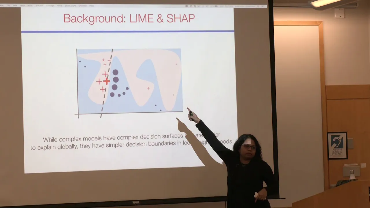
hey guys welcome back to this explainable ai series today we want to have a closer look at one of the most popular methods for explaining black box algorithms which is lime lime stands for local interpretable model agnostic explanations and as the name implies it's model agnostic therefore it can be used for any machine learning model let's first talk about the idea and motivation behind this approach think of the stroke data set we've used in the last video imagine we train a black box algorithm on two features of this data set this could be things like age or body mass index after the training the decision boundary of our complex model could look like this so that's just an example for a new data point if it falls into the blue area we predict no stroke otherwise we predict stroke so the prediction we make is highly non-linear or in other terms there is no easy to explain relationship in how we perform a prediction the model just learned some complex patterns as a combination of those two features if we make a prediction for john now for instance stroke how could we explain to him why our model outputs stroke we cannot easily summarize the whole decision boundary into one explanation the basic idea of lime is that we just zoom into the local area of the individual prediction there we can easily create a simple explanation that makes sense in that local region this way we don't have to worry about the rest of the model and still get a valid explanation why that prediction was made for instance in this example we could say that the prediction was made because the value of feature 2 was small enough to fall on the left side of this dashed line we can also say something about the importance of our variables certainly feature 2 here mainly determines our output class and changes in feature 1 almost have no impact if you've watched the second video of the series about by design interpretable models you probably recall how we can interpret linear regression or simple decision trees to get such kind of explanations lime simply fits a linear interpretable model in that local area which is often also called surrogate it's basically a local approximation of our complex model in this local area so that's the basic idea and now let's have a look at this in more detail lime was presented in the paper on the right and aims to explain any black box model by creating such a local approximation the complex models are complete black boxes and the internals are hidden for lime so it's just based on the inputs and outputs of a model it works on almost any input such as text tabular data images or even graphs usually the domain experts in a certain field let's say medicine have some prior knowledge about the problem for example sports has a positive impact on the overall health if the lime explanation tells us that sports increases the probability of a stroke there's most likely something wrong in our developed model so that helps to build trust and we can assess whether it makes sense or not in the paper they also state that providing explanations improves the acceptance of a predictive algorithm for lyme the only requirement is that the explanations are locally faithful but they might not make sense globally so we just focus on that local area around our prediction now let's have a look at the mathematical optimization problem used in line the idea behind it is actually quite intuitive as already mentioned we want to create a local approximation of our complex model for a specific input for instance we know the properties of john in a tabular format so that would be our input data point x in this optimization formula from the line paper the complex model is denoted with f and the simple model so the local model is denoted with g this simple model small g comes from a set of interpretable models which is denoted with a capital g here capital g is a family of linear models such as linear regression and all its variants in the line paper this family is set to sparse linear models we will further talk about this in a second now this first loss term in our optimization function simply means that we look for an approximation of the complex model f by the simple model g in the neighborhood of our data point x in other terms we want to get a good approximation in that local neighborhoods the third argument pi here defines the local neighborhoods of that data point and is some sort of proximity measure we will see more details in a minute the second loss term is used to regularize the complexity of our simple surrogate model for linear regression for instance a desirable condition could be to have many zero-weighted input features so basically ignoring most of the features and just including a few this makes our explanations more simple for decision tree it would be nice to have a relatively small depth that stays comprehensible for humans so overall this omega is a complexity measure and as this optimization problem is a minimization problem we want to minimize the complexity in summary this loss function says that we look for a simple model g so this is the argument in the arc min that minimizes those two loss terms so it should approximate the complex model in that local area and additionally stay as simple as possible now how is this first loss term calculated so on the right you see the decision boundary of our complex model f again zoomed into that local area of our prediction for john in the first step we simply generate some new data points in the neighborhood of our input data point more specifically we randomly generate data points everywhere but as we will see in a second they will be weighted according to the distance to our input data point as we are just interested in the local area around our input these data points are generated by perturbations so for instance we can slightly increase the h decrease the body mass index and so on this can be achieved by sampling from a normal distribution with the mean and standard deviation for each feature then we get the prediction for these data points using our complex model f so here all the points in the blue area would be predicted as no stroke and the ones on the other side as stroke what we end up with is a new data set we can use to fit a classifier we have the labels which come from the predictions of the complex model f and we have all the feature values which are simply the sample new data points so we minimize the first loss term by simply getting the highest accuracy on that new data set using a simple linear model for a linear regression for instance we minimize the sum of square distances between the predictions and the ground truth in the line paper they use this loss function for optimizing a linear model it's basically the sum of squared distances between the label which comes from the complex model and the prediction of the simple model g additionally the proximity pi is added to weight the loss according to how close a data point is for instance classifying this black data point wrong is not relevant because it falls out of the local neighborhoods in the paper they use an exponential kernel as distance metric so we can think of this like a heat map the points that are close to our input data points are weighteds the most that's how we ensure that the model is locally faithful okay so the first part of that loss function should make sense now what about the omega at the end we said we use it to make sure that our model stays simple in lime a sparse linear model is used the advantage of this is that we additionally take care of the second loss term because sparse linear models aim to produce as many zero weights as possible in practice this can be achieved by using a regularization technique such as done for lasso linear regression for instance this way we ensure to get a simple explanation with only a few relevant variables so that's how we also take care of the second loss term now it's time for some code let's have a look at how we can apply lime on our data set okay so here we are back in vs code first we import a couple of things that data loader i've shown in the last video which simply fetches our data which is a csv file in a tabular format and then uh the random forest classifier which will serve as our black box model in this case as it's an ensemble model that cannot be easily interpreted then we import some metrics like the f1 score and the accuracy score as we have an imbalanced data set it makes sense to also look at recall and precision then we import line tabular which is lime for tabular data and it comes from microsoft's interpret library and as you see it's for black box algorithms and finally we import the show function which helps us to create this interactive plot so in the second cell we load the data set using this load dataset function which simply gets the data as csv from pandas and then we pre-process it using the preprocess function here we do some imputations and one hot encodings and after that we simply split the data set into 20 test data and 80 train data and then we do some over sampling to ensure that our minority class gets more importance in our predictions so let's run those first two cells it's opening our jupiter notebook and now what we do is we create this random forest classifier and fit it using our data and as you can see the accuracy is much better than the previous models we had and also our f1 score is slightly increased it's still not good as it's a relatively complex imbalanced data set but accuracy is pretty good so we can continue with that and now what we do is we use this line tabular class and use our random forest classifier or more specifically the prediction probabilities and pass it our data sets and what we can do now is we can pass the first or the last 20 instances of our data set to make lime explain them locally and what that does is simply creating those local explanations we've just seen that means we fit a local model in the area around each of those 20 data points so let's run this and this will take some time as we have to fit an entirely new model and also sample a data set for each of those 20 data points okay so now it's done and after calling this show function on our local explanations we get this interactive graph which comes from this interpret library so we've trained our random forest classifier with 94 accuracy but can we be sure that the model really uses the right features and works as intended and to better understand that we can now have a look at individual predictions and here we see we have for example actual value of 0 which means no stroke and we have predicted 0.01 as prediction probability so that's also pretty close to zero and the reason for that is so these are the features or the feature values used by our model and the hs has a strongly negative impact because the age is relatively low for a stroke prediction and that's why the prediction is shifted towards no stroke also that the person has no hypertension no heart disease and so on these are reasons why the model says this person is not getting a stroke if we have a look at another prediction here which is also predicting no stroke we see that the h is 22 here so relatively young and that's why the h has a even stronger impact for this individual prediction so as you can see lime can also be used on any black box model to get those kind of explanations we've also seen in a previous video so we've seen how we can use lime to create helpful local explanations to validate our black box model as mentioned before lime can also be applied on other data inputs here's an example for images as you can see depending on the prediction we get different areas in our input which are marked as most important for the prediction here's another example for text data this example shows how helpful lime can be for validating a model on the left we can see that the output class was atheism with 58 probability and in the middle we can see hosting hosts nntp and edu led to a prediction for atheism however with our domain knowledge we know that those words have nothing to do with the religion and that's why we can say there's something going wrong in this model in the paper they also suggest to always look at several local predictions to get a global understanding of what our model is doing so that's it for today i try to keep it short if there's anything else you are interested in just let me know in the comments see you in the next video where we will have a look at another popular method called shep thanks for watching and have a great day
Up Next
96:01
Model Interpretability with LIME & SHAP | Data Science Tutorial
@PyDataTV
40.5K views•2019-02-01

57:48
Secure Multiparty Computation (MPC): Foundations & Challenges
@SimonsInstitute
7.3K views•2015-05-28

6:52
Explainable AI Explained: Introduction to XAI & Interpretable Models
@DeepFindr
89.1K views•2021-02-08

18:41
Neural Networks Explained: Math, Layers, and Learning Fundamentals
@3blue1brown
21.9M views•2017-10-05
Related Study Plans & Knowledge Roadmaps
Structured learning paths in Artificial Intelligence
artificial-intelligence
Aligning LLMs: DPO, TRL & Custom Datasets
01Foundations of Python & Machine Learning
02Transformers and Large Language Models (LLMs)
03Aligning LLMs: SFT and RLHF
+ 3 more learning modules
24h6 modules
Explore Roadmap
artificial-intelligence
Federated Learning: PyTorch, Flower & Privacy
01Python & Machine Learning Foundations
02Deep Learning Basics with PyTorch
03Introduction to Federated Learning
+ 2 more learning modules
35h5 modules
Explore Roadmap
artificial-intelligence
Securing LLMs: Guardrails AI & NeMo Gateway
01Introduction to LLMs, Python, and APIs
02Understanding LLM Vulnerabilities & Threats
03Defending LLMs with Guardrails AI
+ 2 more learning modules
15h5 modules
Explore Roadmap
artificial-intelligence
Building Recommenders: Two-Tower & Vector DBs
01Foundations of Python & Machine Learning Basics
02Introduction to Recommender Systems
03Deep Learning & Representation Learning
+ 3 more learning modules
75h6 modules
Explore Roadmap