













Adversarial examples are inputs that have been carefully modified to cause machine learning models to make confident but incorrect predictions, exploiting the fact that deep neural networks behave approximately linearly in high-dimensional input spaces, allowing attackers to find directions in input space that cause misclassification with minimal perceptible changes to human observers; these vulnerabilities exist across virtually all machine learning algorithms, not just deep learning, and can be mitigated through adversarial training where models are trained on both clean and adversarial examples to improve robustness.
Adversarial Examples & Training in Deep Learning | Stanford Lecture 16
Added:Fundamental concepts of Deep Learning, including feedforward neural networks, Convolutional Neural Networks (CNNs), and the backpropagation algorithm.
The role of loss functions, optimization, and how gradient descent updates model parameters to minimize error.
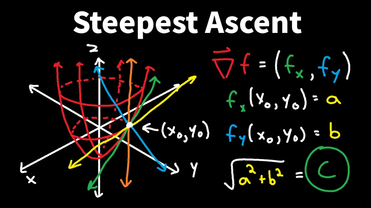
Basic vector calculus and linear algebra, particularly understanding how gradients represent the direction of steepest ascent/descent in high-dimensional spaces.
Standard machine learning evaluation concepts, including training vs. testing distributions, generalization, and decision boundaries.
Mathematical formulation of specific adversarial attack methodologies, such as the Fast Gradient Sign Method (FGSM), Projected Gradient Descent (PGD), and Carlini-Wagner attacks.
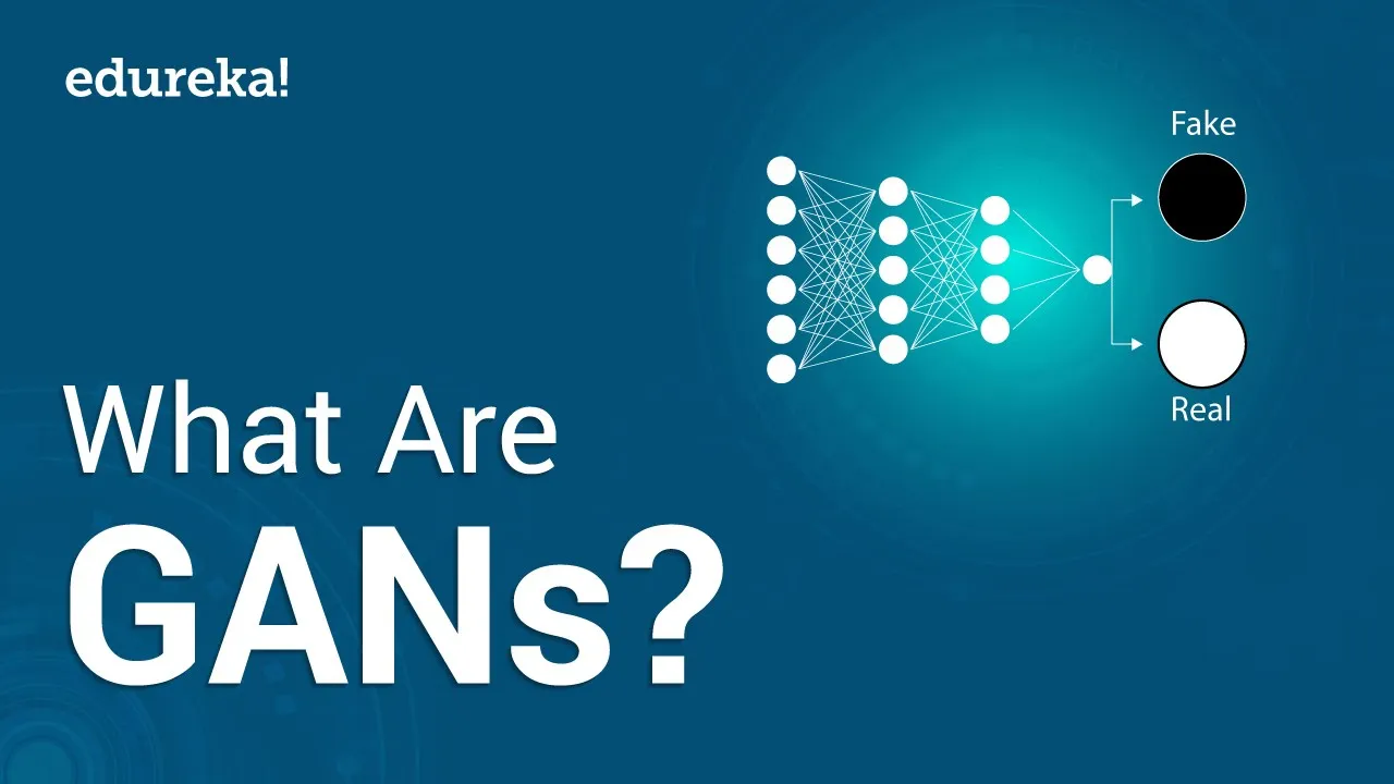
The connection to Generative Adversarial Networks (GANs), which leverage competing neural networks for generative modeling.
Advanced defense strategies and the concept of certifiable robustness, such as randomized smoothing and formal verification techniques.
Real-world security implications and threat modeling in physical-world scenarios, such as fooling autonomous vehicle vision systems or facial recognition systems.
224.7K views2.5Klikes1:21:45Original Release: 2017-08-11
- Okay, sounds like it is.
I'll be telling you about adversarial examples and adversarial training today.
Thank you.
As an overview, I will start off by telling you what adversarial examples are, and then I'll explain why they happen, why it's possible for them to exist.
I'll talk a little bit about how adversarial examples pose real world security threats, that they can actually be used to compromise systems built on machine learning.
I'll tell you what the defenses are so far, but mostly defenses are an open research problem that I hope some of you will move on to tackle.
And then finally I'll tell you how to use adversarial examples to improve other machine learning algorithms even if you want to build a machine learning algorithm that won't face a real world adversary.
Looking at the big picture and the context for this lecture, I think most of you are probably here because you've heard how incredibly powerful and successful machine learning is, that very many different tasks that could not be solved with software before are now solvable thanks to deep learning and convolutional networks and gradient descent.
All of these technologies that are working really well.
Until just a few years ago, these technologies didn't really work.
In about 2013, we started to see that deep learning achieved human level performance at a lot of different tasks.
We saw that convolutional nets could recognize objects and images and score about the same as people in those benchmarks, with the caveat that part of the reason that algorithms score as well as people is that people can't tell Alaskan Huskies from Siberian Huskies very well, but modulo the strangeness of the benchmarks deep learning caught up to about human level performance for object recognition in about 2013.
That same year, we also saw that object recognition applied to human faces caught up to about human level.
That suddenly we had computers that could recognize faces about as well as you or I could recognize faces of strangers.
You can recognize the faces of your friends and family better than a computer, but when you're dealing with people that you haven't had a lot of experience with the computer caught up to us in about 2013.
We also saw that computers caught up to humans for reading type written fonts in photos in about 2013.
It even got the point that we could no longer use CAPTCHAs to tell whether a user of a webpage is human or not because the convolutional network is better at reading obfuscated text than a human is.
So with this context today of deep learning working really well especially for computer vision it's a little bit unusual to think about the computer making a mistake.
Before about 2013, nobody was ever surprised if the computer made a mistake.
That was the rule not the exception, and so today's topic which is all about unusual mistakes that deep learning algorithms make this topic wasn't really a serious avenue of study until the algorithms started to work well most of the time, and now people study the way that they break now that that's actually the exception rather than the rule.
An adversarial example is an example that has been carefully computed to be misclassified.
In a lot of cases we're able to make the new image indistinguishable to a human observer from the original image.
Here, I show you one where we start with a panda.
On the left this is a panda that has not been modified in any way, and the convolutional network trained on the image in that dataset is able to recognize it as being a panda.
One interesting thing is that the model doesn't have a whole lot of confidence in that decision.
It assigns about 60% probability to this image being a panda.
If we then compute exactly the way that we could modify the image to cause the convolutional network to make a mistake we find that the optimal direction to move all the pixels is given by this image in the middle.
To a human it looks a lot like noise.
It's not actually noise.
It's carefully computed as a function of the parameters of the network.
There's actually a lot of structure there.
If we multiply that image of the structured attack by a very small coefficient and add it to the original panda we get an image that a human can't tell from the original panda.
In fact, on this slide there is no difference between the panda on the left and the panda on the right.
When we present the image to convolutional network we use 32-bit floating point values.
The monitor here can only display eight bits of color resolution, and we have made a change that's just barely too small to affect the smallest of those eight bits, but it effects the other 24 of the 32-bit floating point representation, and that little tiny change is enough to fool the convolutional network into recognizing this image of a panda as being a gibbon.
Another interesting thing is that it doesn't just change the class.
It's not that we just barely found the decision boundary and just barely stepped across it.
The convolutional network actually has much more confidence in its incorrect prediction, that the image on the right is a gibbon, than it had for the original being a panda.
On the right, it believes that the image is a gibbon with 99.9% probability, so before it thought that there was about 1/3 chance that it was something other than a panda, and now it's about as certain as it can possibly be that it's a gibbon.
As a little bit of history, people have studied ways of computing attacks to fool different machine learning models since at least about 2004, and maybe earlier.
For a long time this was done in the context of fooling spam detectors.
In about 2013, Battista Biggio found that you could fool neural networks in this way, and around the same time my colleague, Christian Szegedy, found that you could make this kind of attack against deep neural networks just by using an optimization algorithm to search on the input of the image.
A lot of what I'll be telling you about today is my own follow-up work on this topic, but I've spent a lot of my career over the past few years understanding why these attacks are possible and why it's so easy to fool these convolutional networks.
When my colleague, Christian, first discovered this phenomenon independently from Battista Biggio but around the same time, he found that it was actually a result of a visualization he was trying to make.
He wasn't studying security.
He wasn't studying how to fool a neural network.
Instead, he had a convolutional network that could recognize objects very well, and he wants to understand how it worked, so he thought that maybe he could take an image of a scene, for example a picture of a ship, and he could gradually transform that image into something that the network would recognize as being an airplane.
Over the course of that transformation, he could see how the features of the input change.
You might expect that maybe the background 167 00:07:34,360 --> 00:07:37,692 would turn blue to look like the sky behind an airplane, or you might expect that the ship would grow wings to look more like an airplane.
You could conclude from that that the convolution uses the blue sky or uses the wings to recognize airplanes.
That's actually not really what happened at all.
Each of these panels here shows an animation that you read left to right, top to bottom.
Each panel is another step of gradient ascent on the log probability that the input is an airplane according to a convolutional net model, and then we follow the gradient on the input to the image.
You're probably used to following the gradient on the parameters of a model.
You can use the back propagation algorithm to compute the gradient on the input image using exactly the same procedure that you would use to compute the gradient on the parameters.
In this animation of the ship in the upper left, we see five panels that all look basically the same.
Gradient descent doesn't seem to have moved the image at all, but by the last panel the network is completely confident that this is an airplane.
When you first code up this kind of experiment, especially if you don't know what's going to happen, it feels a little bit like you have a bug in your script and you're just displaying the same image over and over again.
The first time I did it, I couldn't believe it was happening, and I had to open up the images in NumPy, and take the difference of them, and make sure that there was actually a non-zero difference in there, but there is.
I show several different animations here of a ship, a car, a cat, and a truck.
The only one where I actually see any change at all is the image of the cat.
The color of the cat's face changes a little bit, and maybe it becomes a little bit more like the color of a metal airplane.
Other than that, I don't see any changes in any of these animations, and I don't see anything very suggestive of an airplane.
So gradient descent, rather than turning the input into an example of an airplane, has found an image that fools the network into thinking that the input is an airplane.
And if we were malicious attackers we didn't even have to work very hard to figure out how to fool the network.
We just asked the network to give us an image of an airplane, and it gave us something that fools it into thinking that the input is an airplane.
When Christian first published this work, a lot of articles came out with titles like, The Flaw Looking At Every Deep Neural Network, or Deep Learning has Deep Flaws.
It's important to remember that these vulnerabilities apply to essentially every machine learning algorithm that we've studied so far.
Some of them like RBF networks and partisan density estimators are able to resist this effect somewhat, but even very simple machine learning algorithms are highly vulnerable to adversarial examples.
In this image, I show an animation of what happens when we attack a linear model, so it's not a deep algorithm at all.
It's just a shallow softmax model.
You multiply by a matrix, you add a vector of bias terms, you apply the softmax function, and you've got your probability distribution over the 10 MNIST classes.
At the upper left, I start with an image of a nine, and then as we move left to right, top to bottom, I gradually transform it to be a zero.
Where I've drawn the yellow box, the model assigns high probability to it being a zero.
I forget exactly what my threshold was for high probability, but I think it was around 0.9 or so.
Then as we move to the second row, I transform it into a one, and the second yellow box indicates where we've successfully fooled the model into thinking it's a one with high probability.
And then as you read the rest of the yellow boxes left to right, top to bottom, we go through the twos, threes, fours, and so on, until finally at the lower right we have a nine that has a yellow box around it, and it actually looks like a nine, but in this case the only reason it actually looks like a nine is that we started the whole process with a nine.
We successfully swept through all 10 classes of MNIST without substantially changing the image of the digit in any way that would interfere with human recognition.
This linear model was actually extremely easy to fool.
Besides linear models, we've also seen that we can fool many different kinds of linear models including logistic regression and SVMs.
We've also found that we can fool decision trees, and to a lesser extent, nearest neighbors classifiers.
We wanted to explain exactly why this happens.
Back in about 2014, after we'd published the original paper where we'd said that these problems exist, we were trying to figure out why they happen.
When we wrote our first paper, we thought that basically this is a form of overfitting, that you have a very complicated deep neural network, it learns to fit the training set, its behavior on the test set is somewhat undefined, and then it makes random mistakes that an attacker can exploit.
Let's walk through what that story looks like somewhat concretely.
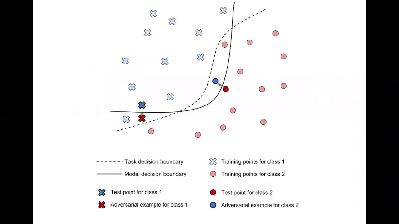
I have here a training set of three blue X's and three green O's.
We want to make a classifier that can recognize X's and recognize O's.
We have a very complicated classifier that can easily fit the training set, so we represent everywhere it believes X's should be with blobs of blue color, and I've drawn a blob of blue around all of the training set X's, so it correctly classifies the training set.
It also has a blob of green mass showing where the O's are, and it successfully fits all of the green training set O's, but then because this is a very complicated function and it has just way more parameters than it actually needs to represent the training task, it throws little blobs of probability mass around the rest of space randomly.
On the left there's a blob of green space that's kind of near the training set X's, and I've drawn a red X there to show that maybe this would be an adversarial example where we expect the classification to be X, but the model assigns O.
On the right, I've shown that there's a red O where we have another adversarial example.
We're very near the other O's.
We might expect the model to assign this class to be an O, and yet because it's drawn blue mass there it's actually assigning it to be an X.
If overfitting is really the story then each adversarial example is more or less the result of bad luck and also more or less unique.
If we fit the model again or we fit a slightly different model we would expect to make different random mistakes on this points that are off the training set, but that was actually not what we found at all.
We found that many different models would misclassify the same adversarial examples, and they would assign the same class to them.
We also found that if we took the difference between an original example and an adversarial example then we had a direction in input space and we could add that same offset vector to any clean example, and we would almost always get an adversarial example as a result.
So we started to realize that there was systematic effect going on here, not just a random effect.
That led us to another idea which is that adversarial examples might actually be more like underfitting rather than overfitting.
They might actually come from the model being too linear.
Here I draw the same task again where we have the same manifold of O's and the same line of X's, and this time I fit a linear model to the data set rather than fitting a high capacity, non-linear model to it.
We see that we get a dividing hyperplane running in between the two classes.
This hyperplane doesn't really capture the true structure of the classes.
The O's are clearly arranged in a C-shaped manifold.
If we keep walking past the end of the O's, we've crossed the decision boundary and we've drawn a red O where even though we're very near the decision boundary and near other O's we believe that it is now an X.
Similarly we can take steps that go from near X's to just over the line that are classified as O's.
Another thing that's somewhat unusual about this plot is that if we look at the lower left or upper right corners these corners are very confidently classified as being X's on the lower left or O's on the upper right even though we've never seen any data over there at all.
The linear model family forces the model to have very high confidence in these regions that are very far from the decision boundary.
We've seen that linear models can actually assign really unusual confidence as you move very far from the decision boundary, even if there isn't any data there, but are deep neural networks actually anything like linear models?
Could linear models actually explain anything about how it is that deep neural nets fail?
It turns out that modern deep neural nets are actually very piecewise linear, so rather than being a single linear function they are piecewise linear with maybe not that many linear pieces.
If we use rectified linear units then the mapping from the input image to the output logits is literally a piecewise linear function.
By the logits I mean the un-normalized log probabilities before we apply the softmax op at the output of the model.
There are other neural networks like maxout networks that are also literally piecewise linear.
And then there are several that become very close to it.
Before rectified linear units became popular most people used to use sigmoid units of one form or another either logistic sigmoid or hyperbolic tangent units.
These sigmoidal units have to be carefully tuned, especially at initialization so that you spend most of your time near the center of the sigmoid where the sigmoid is approximately linear.
Then finally, the LSTM, a kind of recurrent network that is one of the most popular recurrent networks today, uses addition from one time step to the next in order to accumulate and remember information over time.
Addition is a particularly simple form of linearity, so we can see that the interaction from a very distant time step in the past and the present is highly linear within an LSTM.
Now to be clear, I'm speaking about the mapping from the input of the model to the output of the model.
That's what I'm saying is close to being linear or is piecewise linear with relatively few pieces.
The mapping from the parameters of the network to the output of the network is non-linear because the weight matrices at each layer of the network are multiplied together.
So we actually get extremely non-linear reactions between parameters and the output.
That's what makes training a neural network so difficult.
But the mapping from the input to the output is much more linear and predictable, and it means that optimization problems that aim to optimize the input to the model are much easier than optimization problems that aim to optimize the parameters.
If we go and look for this happening in practice we can take a convolutional network and trace out a one-dimensional path through its input space.
So what we're doing here is we're choosing a clean example.
It's an image of a white car on a red background, and we are choosing a direction that will travel through space.
We are going to have a coefficient epsilon that we multiply by this direction.
When epsilon is negative 30, like at the left end of the plot, we're subtracting off a lot of this unit vector direction.
When epsilon is zero, like in the middle of the plot, we're visiting the original image from the data set, and when epsilon is positive 30, like at the right end of the plot, we're adding this direction onto the input.
In the panel on the left, I show you an animation where we move from epsilon equals negative 30 as up to epsilon equals positive 30.
You read the animation left to right, top to bottom, and everywhere that there's a yellow box the input has correctly recognized as being a car.
On the upper left, you see that it looks mostly blue.
On the lower right, it's hard to tell what's going on.
It's kind of reddish and so on.
In the middle row, just after where the yellow boxes end you can see pretty clearly that it's a car on a red background, though the image is small on these slides.
What's interesting to look at here is the logits that the model outputs.
This is a deep convolutional rectified linear unit network.
Because it uses rectified linear units, we know that the output is a piecewise linear function of the input to the model.
The main question we're asking by making this plot is how many different pieces does this piecewise linear function have if we look at one particular cross section.
You might think that maybe a deep net is going to represent some extremely wiggly complicated function with lots and lots of linear pieces no matter which cross section you look in.
Or we might find that it has more or less two pieces for each function we look at.
Each of the different curves on this plot is the logits for a different class.
We see that out at the tails of the plot that the frog class is the most likely, and the frog class basically looks like a big v-shaped function.
The logits for the frog class become very high when epsilon is negative 30 or positive 30, and they drop down and become a little bit negative when epsilon is zero.
The car class, listed as automobile here, it's actually high in the middle, and the car is correctly recognized.
As we sweep out to very negative epsilon, the logits for the car class do increase, but they don't increase nearly as quickly as the logits for the frog class.
So, we've found a direction that's associated with the frog class and as we follow it out to a relatively large perturbation, we find that the model extrapolates linearly and begins to make a very unreasonable prediction that the frog class is extremely likely just because we've moved for a long time in this direction that was locally associated with the frog class being more likely.
When we actually go and construct adversarial examples, we need to remember that we're able to get quite a large perturbation without changing the image very much as far as a human being is concerned.
So here I show you a handwritten digit three, and I'm going to change it in several different ways, and all of these changes have the same L2 norm perturbation.
In the top row, I'm going to change the three into a seven just by looking for the nearest seven in the training set.
The difference between those two is this image that looks a little bit like the seven wrapped in some black lines.
So here white pixels in the middle image in the perturbation column, the white pixels represent adding something and black pixels represent subtracting something as you move from the left column to the right column.
So when we take the three and we apply this perturbation that transforms it into a seven, we can measure the L2 norm of that perturbation.
And it turns out to have an L2 norm of 3.96.
That gives you kind of a reference for how big these perturbations can be.
In the middle row, we apply a perturbation of exactly the same size, but with the direction chosen randomly.
In this case we don't actually change the class of the three at all, we just get some random noise that didn't really change the class.
A human could still easily read it as being a three.
And then finally at the very bottom row, we take the three and we just erase a piece of it with a perturbation of the same norm and we turn it into something that doesn't have any class at all.
It's not a three, it's not a seven, it's just a defective input.
All of these changes can happen with the same L2 norm perturbation.
And actually a lot of the time with adversarial examples, you make perturbations that have an even larger L2 norm.
What's going on is that there are several different pixels in the image, and so small changes to individual pixels can add up to relatively large vectors.
For larger datasets like ImageNet, where there's even more pixels, you can make very small changes to each pixel that travel very far in vector space as measured by the L2 norm.
That means that you can actually make changes that are almost imperceptible but actually move you really far and get a large dot product with the coefficients of the linear function that the model represents.
It also means that when we're constructing adversarial examples, we need to make sure that the adversarial example procedure isn't able to do what happened in the top row of this slide here.
So in the top row of this slide, we took the three and we actually just changed it into a seven.
So when the model says that the image in the upper right is a seven, it's not a mistake.
We actually just changed the input class.
When we build adversarial examples, we want to make sure that we're measuring real mistakes.
If we're experimenters studying how easy a network is to fool, we want to make sure that we're actually fooling it and not just changing the input class.
And if we're an attacker, we actually want to make sure that we're causing misbehavior in the system.
To do that, when we build adversarial examples, we use the maxnorm to constrain the perturbation.
Basically this says that no pixel can change by more than some amount epsilon.
So the L2 norm can get really big, but you can't concentrate all the changes for that L2 norm to erase pieces of the digit, like in the bottom row here we erased the top of a three.
One very fast way to build an adversarial example is just to take the gradient of the cost that you used to train the network with respect to the input, and then take the sign of that gradient.
The sign is essentially enforcing the maxnorm constraint.
You're only allowed to change the input by up to epsilon at each pixel, so if you just take the sign it tells you whether you want to add epsilon or subtract epsilon in order to hurt the network.
You can view this as taking the observation that the network is more or less linear, as we showed on this slide, and using that to motivate building a first order Taylor series approximation of the neural network's cost.
And then subject to that Taylor series approximation, we want to maximize the cost following this maxnorm constraint.
And that gives us this technique that we call the fast gradient sign method.
If you want to just get your hands dirty and start making adversarial examples really quickly, or if you have an algorithm where you want to train on adversarial examples in the inner loop of learning, this method will make adversarial examples for you very, very quickly.
In practice you should also use other methods, like Nicholas Carlini's attack based on multiple steps of the Adam optimizer, to make sure that you have a very strong attack that you bring out when you think you have a model that might be more powerful.
A lot of the time people find that they can defeat the fast gradient sign method and think that they've built a successful defense, but then when you bring out a more powerful method that takes longer to evaluate, they find that they can't overcome the more computationally expensive attack.
I've told you that adversarial examples happen because the model is very linear.
And then I told you that we could use this linearity assumption to build this attack, the fast gradient sign method.
This method, when applied to a regular neural network that doesn't have any special defenses, will get over a 99% attack success rate.
So that seems to confirm, somewhat, this hypothesis that adversarial examples come from the model being far too linear and extrapolating in linear fashions when it shouldn't.
Well we can actually go looking for some more evidence.
My friend David Warde-Farley and I built these maps of the decision boundaries of neural networks.
And we found that they are consistent with the linearity hypothesis.
So the FGSM is that attack method that I described in the previous slide, where we take the sign of the gradient.
We'd like to build a map of a two-dimensional cross section of input space and show which classes are assigned to the data at each point.
In the grid on the right, each different cell, each little square within the grid, is a map of a CIFAR-10 classifier's decision boundary, with each cell corresponding to a different CIFAR-10 testing sample.
On the left I show you a little legend where you can understand what each cell means.
The very center of each cell corresponds to the original example from the CIFAR-10 dataset with no modification.
As we move left to right in the cell, we're moving in the direction of the fast gradient sign method attack.
So just the sign of the gradient.
As we move up and down within the cell, we're moving in a random direction that's orthogonal to the fast gradient sign method direction.
So we get to see a cross section, a 2D cross section of CIFAR-10 decision space.
At each pixel within this map, we plot a color that tells us which class is assigned there.
We use white pixels to indicate that the correct class was chosen, and then we used different colors to represent all of the other incorrect classes.
You can see that in nearly all of the grid cells on the right, roughly the left half of the image is white.
So roughly the left half of the image has been correctly classified.
As we move to the right, we see that there is usually a different color on the right half.
And the boundaries between these regions are approximately linear.
What's going on here is that the fast gradient sign method has identified a direction where if we get a large dot product with that direction we can get an adversarial example.
And from this we can see that adversarial examples live more or less in linear subspaces.
When we first discovered adversarial examples, we thought that they might live in little tiny pockets.
In the first paper we actually speculated that maybe they're a little bit like the rational numbers, hiding out finely tiled among the real numbers, with nearly every real number being near a rational number.
We thought that because we were able to find an adversarial example corresponding to every clean example that we loaded into the network.
After doing this further analysis, we found that what's happening is that every real example is near one of these linear decision boundaries where you cross over into an adversarial subspace.
And once you're in that adversarial subspace, all the other points nearby are also adversarial examples that will be misclassified.
This has security implications because it means you only need to get the direction right.
You don't need to find an exact coordinate in space.
You just need to find a direction that has a large dot product with the sign of the gradient.
And once you move more or less approximately in that direction, you can fool the model.
We also made another cross section where after using the left-right axis as the fast gradient sign method, we looked for a second direction that has high dot product with the gradient so we could make both axes adversarial.
And in this case you see that we get linear decision boundaries.
They're now oriented diagonally rather than vertically, but you can see that there's actually this two-dimensional subspace of adversarial examples that we can cross into.
Finally it's important to remember that adversarial examples are not noise.
You can add a lot of noise to an adversarial example and it will stay adversarial.
You can add a lot of noise to a clean example and it will stay clean.
Here we make random cross sections where both axes are randomly chosen directions.
And you see that on CIFAR-10, most of the cells are completely white, meaning that they're correctly classified to start with, and when you add noise they stay correctly classified.
We also see that the model makes some mistakes because this is the test set.
And generally if a test example starts out misclassified, adding the noise doesn't change it.
There are a few exceptions where, if you look in the third row, third column, noise actually can make the model misclassify the example for especially large noise values.
And there's even some where, in the top row there's one example you can see where the model is misclassifying the test example to start with but then noise can change it to be correctly classified.
For the most part, noise has very little effect on the classification decision compared to adversarial examples.
What's going on here is that in high dimensional spaces, if you choose some reference vector and then you choose a random vector in that high dimensional space, the random vector will, on average, have zero dot product with the reference vector.
So if you think about making a first order Taylor series approximation of your cost, and thinking about how your Taylor series approximation predicts that random vectors will change your cost.
You see that random vectors on average have no effect on the cost.
But adversarial examples are chosen to maximize it.
In these plots we looked in two dimensions.
More recently, Florian Tramer here at Stanford got interested in finding out just how many dimensions there are to these subspaces where the adversarial examples lie in a thick contiguous region.
And we came up with an algorithm together where you actually look for several different orthogonal vectors that all have a large dot product with the gradient.
By looking in several different orthogonal directions simultaneously, we can map out this kind of polytope where many different adversarial examples live.
We found out that this adversarial region has on average about 25 dimensions.
If you look at different examples you'll find different numbers of adversarial dimensions.
But on average on MNIST we found it was about 25.
So what's interesting here is the dimensionality actually tells you something about how likely you are to find an adversarial example by generating random noise.
If every direction were adversarial, then any change would cause a misclassification.
If most of the directions were adversarial, then random directions would end up being adversarial just by accident most of the time.
And then if there was only one adversarial direction, you'd almost never find that direction just by adding random noise.
When there's 25 you have a chance of doing it sometimes.
Another interesting thing is that different models will often misclassify the same adversarial examples.
The subspace dimensionality of the adversarial subspace relates to that transfer property.
The larger the dimensionality of the subspace, the more likely it is that the subspaces for two models will intersect.
So if you have two different models that have a very large adversarial subspace, you know that you can probably transfer adversarial examples from one to the other.
But if the adversarial subspace is very small, then unless there's some kind of really systematic effect forcing them to share exactly the same subspace, it seems less likely that you'll be able to transfer examples just due to the subspaces randomly aligning.
A lot of the time in the adversarial example research community, we refer back to the story of Clever Hans.
This comes from an essay by Bob Sturm called Clever Hans, Clever Algorithms.
Because Clever Hans is a pretty good metaphor for what's happening with machine learning algorithms.
So Clever Hans was a horse that lived in the early 1900s.
His owner trained him to do arithmetic problems.
So you could ask him, "Clever Hans, "what's two plus one?"
And he would answer by tapping his hoof.
And after the third tap, everybody would start cheering and clapping and looking excited because he'd actually done an arithmetic problem.
Well it turned out that he hadn't actually learned to do arithmetic.
But it was actually pretty hard to figure out what was going on.
His owner was not trying to defraud anybody, his owner actually believed he could do arithmetic.
And presumably Clever Hans himself was not trying to trick anybody.
But eventually a psychologist examined him and found that if he was put in a room alone without an audience, and the person asking the questions wore a mask, he couldn't figure out when to stop tapping.
You'd ask him, "Clever Hans, "what's one plus one?"
And he'd just [knocking] keep staring at your face, waiting for you to give him some sign that he was done tapping.
So everybody in this situation was trying to do the right thing.
Clever Hans was trying to do whatever it took to get the apple that his owner would give him when he answered an arithmetic problem.
His owner did his best to train him correctly with real arithmetic questions and real rewards for correct answers.
And what happened was that Clever Hans inadvertently focused on the wrong cue.
He found this cue of people's social reactions that could reliably help him solve the problem, but then it didn't generalize to a test set where you intentionally took that cue away.
It did generalize to a naturally occurring test set, where he had an audience.
So that's more or less what's happening with machine learning algorithms.
They've found these very linear patterns that can fit the training data, and these linear patterns even generalize to the test data.
They've learned to handle any example that comes from the same distribution as their training data.
But then if you shift the distribution that you test them on, if a malicious adversary actually creates examples that are intended to fool them, they're very easily fooled.
In fact we find that modern machine learning algorithms are wrong almost everywhere.
We tend to think of them as being correct most of the time, because when we run them on naturally occurring inputs they achieve very high accuracy percentages.
But if we look instead of as the percentage of samples from an IID test set, if we look at the percentage of the space in RN that is correctly classified, we find that they misclassify almost everything and they behave reasonably only on a very thin manifold surrounding the data that we train them on.
In this plot, I show you several different examples of Gaussian noise that I've run through a CIFAR-10 classifier.
Everywhere that there is a pink box, the classifier thinks that there is something rather than nothing.
I'll come back to what that means in a second.
Everywhere that there is a yellow box, one step of the fast gradient sign method was able to persuade the model that it was looking specifically at an airplane.
I chose the airplane class because it was the one with the lowest success rate.
It had about a 25% success rate.
That means an attacker would need four chances to get noise recognized as an airplane on this model.
An interesting thing, and appropriate enough given the story of Clever Hans, is that this model found that about 70% of RN was classified as a horse.
So I mentioned that this model will say that noise is something rather than nothing.
And it's actually kind of important to think about how we evaluate that.
If you have a softmax classifier, it has to give you a distribution over the n different classes that you train it on.
So there's a few ways that you can argue that the model is telling you that there's something rather than nothing.
One is you can say, if it assigns something like 90% to one particular class, that seems to be voting for that class being there.
We'd much rather see it give us something like a uniform distribution saying this noise doesn't look like anything in the training set so it's equally likely to be a horse or a car.
And that's not what the model does.
It'll say, this is very definitely a horse.
Another thing that you can do is you can replace the last layer of the model.
For example, you can use a sigmoid output for each class.
And then the model is actually capable of telling you that any subset of classes is present.
It could actually tell you that an image is both a horse and a car.
And what we would like it to do for the noise is tell us that none of the classes is present, that all of the sigmoids should have a value of less than 1/2.
And 1/2 isn't even particularly a low threshold.
We could reasonably expect that all of the sigmoids would be less than 0.01 for such a defective input as this.
But what we find instead is that the sigmoids tend to have at least one class present just when we run Gaussian noise of sufficient norm through the model.
We've also found that we can do adversarial examples for reinforcement learning.
And there's a video for this.
I'll upload the slides after the talk and you can follow the link.
Unfortunately I wasn't able to get the WiFi to work so I can't show you the video animated.
But I can describe basically what's going on from this still here.
There's a game Seaquest on Atari where you can train reinforcement learning agents to play that game.
And you can take the raw input pixels and you can take the fast gradient sign method or other attacks that use other norms besides the max norm, and compute perturbations that are intended to change the action that the policy would select.
So the reinforcement learning policy, you can think of it as just being like a classifier that looks at a frame.
And instead of categorizing the input into a particular category, it gives you a softmax distribution over actions to take.
So if we just take that and say that the most likely action should have its accuracy be decreased by the adversary.
Sorry, to have its probability be decreased by the adversary, you'll get these perturbations of input frames that you can then apply and cause the agent to play different actions than it would have otherwise.
And using this you can make the agent play Seaquest very, very badly.
It's maybe not the most interesting possible thing.
What we'd really like is an environment where there are many different reward functions available for us to study.
So for example, if you had a robot that was intended to cook scrambled eggs, and you had a reward function measuring how well it's cooking scrambled eggs, and you had another reward function measuring how well it's cooking chocolate cake, it would be really interesting if we could make adversarial examples that cause the robot to make a chocolate cake when the user intended for it to make scrambled eggs.
That's because it's very difficult to succeed at something and it's relatively straightforward to make a system fail.
So right now, adversarial examples for RL are very good at showing that we can make RL agents fail.
But we haven't yet been able to hijack them and make them do a complicated task that's different from what their owner intended.
Seems like it's one of the next steps in adversarial example research though.
If we look at high-dimension linear models, we can actually see that a lot of this is very simple and straightforward.
Here we have a logistic regression model that classifies sevens and threes.
So the whole model can be described just by a weight vector and a single scalar bias term.
We don't really need to see the bias term for this exercise.
If you look on the left I've plotted the weights that we used to discriminate sevens and threes.
The weights should look a little bit like the difference between the average seven and the average three.
And then down at the bottom we've taken the sign of the weights.
So the gradient for a logistic regression model is going to be proportional to the weights.
And then the sign of the weights gives you essentially the sign of the gradient.
So we can do the fast gradient sign method to attack this model just by looking at its weights.
In the examples in the panel that's the second column from the left we can see clean examples.
And then on the right we've just added or subtracted this image of the sign of the weights off of them.
To you and me as human observers, the sign of the weights is just like garbage that's in the background, and we more or less filter it out.
It doesn't look particularly interesting to us.
It doesn't grab our attention.
To the logistic regression model this image of the sign of the weights is the most salient thing that could ever appear in the image.
When it's positive it looks like the world's most quintessential seven.
When it's negative it looks like the world's most quintessential three.
And so the model makes its decision almost entirely based on this perturbation we added to the image, rather than on the background.
You could also take this same procedure, and my colleague Andrej at OpenAI showed how you can modify the image on ImageNet using this same approach, and turn this goldfish into a daisy.
Because ImageNet is much higher dimensional, you don't need to use quite as large of a coefficient on the image of the weights.
So we can make a more persuasive fooling attack.
You can see that this same image of the weights, when applied to any different input image, will actually reliably cause a misclassification.
What's going on is that there are many different classes, and it means that if you choose the weights for any particular class, it's very unlikely that a new test image will belong to that class.
So on ImageNet, if we're using the weights for the daisy class, and there are 1,000 different classes, then we have about a 99.9% chance that a test image will not be a daisy.
If we then go ahead and add the weights for the daisy class to that image, then we get a daisy, and because that's not the correct class, it's a misclassification.
So there's a paper at CVPR this year called Universal Adversarial Perturbations that expands a lot more on this observation that we had going back in 2014.
But basically these weight vectors, when applied to many different images, can cause misclassification in all of them.
I've spent a lot of time telling you that these linear models are just terrible, and at some point you've probably been hoping I would give you some sort of a control experiment to convince you that there's another model that's not terrible.
So it turns out that some quadratic models actually perform really well.
In particular a shallow RBF network is able to resist adversarial perturbations very well.
Earlier I showed you an animation where I took a nine and I turned it into a zero, one, two, and so on, without really changing its appearance at all.
And I was able to fool a linear softmax regression classifier.
Here I've got an RBF network where it outputs a separate probability of each class being absent or present, and that probability is given by e to the negative square of the difference between a template image and the input image.
And if we actually follow the gradient of this classifier, it does actually turn the image into a zero, a one, a two, a three, and so on, and we can actually recognize those changes.
The problem is, this classifier does not get very good accuracy on the training set.
It's a shallow model.
It's basically just a template matcher.
It is literally a template matcher.
And if you try to make it more sophisticated by making it deeper, it turns out that the gradient of these RBF units is zero, or very near zero, throughout most of RN.
So they're extremely difficult to train, even with batch normalization and methods like that.
I haven't managed to train a deep RBF network yet.
But I think if somebody comes up with better hyperparameters or a new, more powerful optimization algorithm, it might be possible to solve the adversarial example problem by training a deep RBF network where the model is so nonlinear and has such wide flat areas that the adversary is not able to push the cost uphill just by making small changes to the model's input.
One of the things that's the most alarming about adversarial examples is that they generalize from one dataset to another and one model to another.
Here I've trained two different models on two different training sets.
The training sets are tiny in both cases.
It's just MNIST three versus seven classification, and this is really just for the purpose of making a slide.
If you train a logistic regression model on the digits shown in the left panel, you get the weights shown on the left in the lower panel.
If you train a logistic regression model on the digits shown in the upper right, you get the weights shown on the right in the lower panel.
So you've got two different training sets and we learn weight vectors that look very similar to each other.
That's just because machine learning algorithms generalize.
You want them to learn a function that's somewhat independent of the data that you train them on.
It shouldn't matter which particular training examples you choose.
If you want to generalize from the training set to the test set, you've also got to expect that different training sets will give you more or less the same result.
And that means that because they've learned more or less similar functions, they're vulnerable to similar adversarial examples.
An adversary can compute an image that fools one and use it to fool the other.
In fact we can actually go ahead and measure the transfer rate between several different machine learning techniques, not just different data sets.
Nicolas Papernot and his collaborators have spent a lot of time exploring this transferability effect.
And they found that for example, logistic regression makes adversarial examples that transfer to decision trees with 87.4% probability.
Wherever you see dark squares in this matrix, that shows that there's a high amount of transfer.
That means that it's very possible for an attacker using the model on the left to create adversarial examples for the model on the right.
The procedure overall is that, suppose the attacker wants to fool a model that they don't actually have access to.
They don't know the architecture that's used to train the model.
They may not even know which algorithm is being used.
They may not know whether they're attacking a decision tree or a deep neural net.
And they also don't know the parameters of the model that they're going to attack.
So what they can do is train their own model that they'll use to build the attack.
There's two different ways you can train your own model.
One is you can label your own training set for the same task that you want to attack.
Say that somebody is using an ImageNet classifier, and for whatever reason you don't have access to ImageNet, you can take your own photos and label them, train your own object recognizer.
It's going to share adversarial examples with an ImageNet model.
The other thing you can do is, say that you can't afford to gather your own training set.
What you can do instead is if you can get limited access to the model where you just have the ability to send inputs to the model and observe its outputs, then you can send those inputs, observe the outputs, and use those as your training set.
This'll work even if the output that you get from the target model is only the class label that it chooses.
A lot of people read this and assume that you need to have access to all the probability values it outputs.
But even just the class labels are sufficient.
So once you've used one of these two methods, either gather your own training set or observing the outputs of a target model, you can train your own model and then make adversarial examples for your model.
Those adversarial examples are very likely to transfer and affect the target model.
So you can then go and send those out and fool it, even if you didn't have access to it directly.
We've also measured the transferability across different data sets, and for most models we find that they're kind of in an intermediate zone where different data sets will result in a transfer rate of, like, 60% to 80%.
There's a few models like SVMs that are very data dependent because SVMs end up focusing on a very small subset of the training data to form their final decision boundary.
But most models that we care about are somewhere in the intermediate zone.
Now that's just assuming that you rely on the transfer happening naturally.
You make an adversarial example and you hope that it will transfer to your target.
What if you do something to stack the deck in your favor and improve the odds that you'll get your adversarial examples to transfer?
Dawn Song's group at UC Berkeley studied this.
They found that if they take an ensemble of different models and they use gradient descent to search for an adversarial example that will fool every member of their ensemble, then it's extremely likely that it will transfer and fool a new machine learning model.
So if you have an ensemble of five models, you can get it to the point where there's essentially a 100% chance that you'll fool a sixth model out of the set of models that they compared.
They looked at things like ResNets of different depths, VGG, and GoogLeNet.
So in the labels for each of the different rows you can see that they made ensembles that lacked each of these different models, and then they would test it on the different target models.
So like if you make an ensemble that omits GoogLeNet, you have only about a 5% chance of GoogLeNet correctly classifying the adversarial example you make for that ensemble.
If you make an ensemble that omits ResNet-152, in their experiments they found that there was a 0% chance of ResNet-152 resisting that attack.
That probably indicates they should have run some more adversarial examples until they found a non-zero success rate, but it does show that the attack is very powerful.
And then when you go look into intentionally cause the transfer effect, you can really make it quite strong.
A lot of people often ask me if the human brain is vulnerable to adversarial examples.
And for this lecture I can't use copyrighted material, but there's some really hilarious things on the Internet if you go looking for, like, the fake CAPTCHA with images of Mark Hamill, you'll find something that my perception system definitely can't handle.
So here's another one that's actually published with a license where I was confident I'm allowed to use it.
You can look at this image of different circles here, and they appear to be intertwined spirals.
But in fact they are concentric circles.
The orientation of the edges of the squares is interfering with the edge detectors in your brain, making it look like the circles are spiraling.
So you can think of these optical illusions as being adversarial examples in the human brain.
What's interesting is that we don't seem to share many adversarial examples in common with machine learning models.
Adversarial examples transfer extremely reliably between different machine learning models, especially if you use that ensemble trick that was developed at UC Berkeley.
But those adversarial examples don't fool us.
It tells us that we must be using a very different algorithm or model family than current convolutional networks.
We don't really know what the difference is yet, but it would be very interesting to figure that out.
It seems to suggest that studying adversarial examples could tell us how to significantly improve our existing machine learning models.
Even if you don't care about having an adversary, we might figure out something or other about how to make machine learning algorithms deal with ambiguity and unexpected inputs more like a human does.
If we actually want to go out and do attacks in practice, there's started to be a body of research on this subject.
Nicolas Papernot showed that he could use the transfer effect to fool classifiers hosted by MetaMind, Amazon, and Google.
So these are all just different machine learning APIs where you can upload a dataset and the API will train the model for you.
And then you don't actually know, in most cases, which model is trained for you.
You don't have access to its weights or anything like that.
So Nicolas would train his own copy of the model using the API, and then build a model on his own personal desktop where he could fool the API hosted model.
Later, Berkeley showed you could fool Clarifai in this way.
Yeah?
- [Man] What did you mean when you said machine having adversarial models don't generally fool us?
Because I thought that was part of the point that we generally do machine-generated adversarial models where just a few pixels change.
- Oh, so if we look at, for example, like this picture of the panda.
To us it looks like a panda.
To most machine learning models it looks like a gibbon.
And so this change isn't interfering with our brains, but it fools reliably with lots of different machine learning models.
I saw somebody actually took this image of the perturbation out of our paper, and they pasted it on their Facebook profile picture to see if it could interfere with Facebook recognizing them.
And they said that it did.
I don't think that Facebook has a gibbon tag though, so we don't know if they managed to make it think that they were a gibbon.
And one of the other things that you can do that's of fairly high practical significance is you can actually fool malware detectors.
Catherine Gross at the University of Saarland wrote a paper about this.
And there's starting to be a few others.
There's a model called MalGAN that actually uses a GAN to generate adversarial examples for malware detectors.
Another thing that matters a lot if you are interested in using these attacks in the real world and defending against them in the real world is that a lot of the time you don't actually have access to the digital input to a model.
If you're interested in the perception system for a self-driving car or a robot, you probably don't get to actually write to the buffer on the robot itself.
You just get to show the robot objects that it can see through a camera lens.
So my colleague Alexey Kurakin and Samy Bengio and I wrote a paper where we studied if we can actually fool an object recognition system running on a phone, where it perceives the world through a camera.
Our methodology was really straightforward.
We just printed out several pictures of adversarial examples.
And we found that the object recognition system run by the camera was fooled by them.
The system on the camera is actually different from the model that we used to generate the adversarial examples.
So we're showing not just transfer across the changes that happen when you use the camera, we're also showing that those transfer across the model that you use.
So the attacker could conceivably fool a system that's deployed in a physical agent, even if they don't have access to the model on that agent and even if they can't interface directly with the agent but just subtly modify objects that it can see in its environment.
Yeah?
- [Man] Why does the, for the low quality camera image noise not affect the adversarial example?
Because that's what one would expect.
- Yeah, so I think a lot of that comes back to the maps that I showed earlier.
If you cross over the boundary into the realm of adversarial examples, they occupy a pretty wide space and they're very densely packed in there.
So if you jostle around a little bit, you're not going to recover from the adversarial attack.
If the camera noise, somehow or other, was aligned with the negative gradient of the cost, then the camera could take a gradient descent step downhill and rescue you from the uphill step that the adversary took.
But probably the camera's taking more or less something that you could model as a random direction.
Like clearly when you use the camera more than once it's going to do the same thing each time, but from the point of view of how that direction relates to the image classification problem, it's more or less a random variable that you sample once.
And it seems unlikely to align exactly with the normal to this class boundary.
There's a lot of different defenses that we'd like to build.
And it's a little bit disappointing that I'm mostly here to tell you about attacks.
I'd like to tell you how to make your systems more robust.
But basically every attack we've tried has failed pretty badly.
And in fact, even when people have published that they successfully defended.
Well, there's been several papers on arXiv over the last several months.
Nicholas Carlini at Berkeley just released a paper where he shows that 10 of those defenses are broken.
So this is a really, really hard problem.
You can't just make it go away by using traditional regularization techniques.
Particular, generative models are not enough to solve the problem.
A lot of people say, "Oh the problem that's going on here "is you don't know anything about the distribution "over the input pixels.
"If you could just tell "whether the input is realistic or not "then you'd be able to resist it."
It turns out that what's going on here is what matters more than getting the right distributions over the inputs x, is getting the right posterior distribution over the class of labels y given inputs x.
So just using a generative model is not enough to solve the problem.
I think a very carefully designed generative model could possibly do it.
Here I show two different modes of a bimodal distribution, and we have two different generative models that try to capture these modes.
On the left we have a mixture of two Gaussians.
On the right we have a mixture of two Laplacians.
You can not really tell the difference visually between the distribution they impose over x, and the difference in the likelihood they assign to the training data is negligible.
But the posterior distribution they assign over classes is extremely different.
On the left we get a logistic regression classifier that has very high confidence out in the tails of the distribution where there is never any training data.
On the right, with the Laplacian distribution, we level off to more or less 50-50.
Yeah?
[speaker drowned out] The issue is that it's a nonstationary distribution.
So if you train it to recognize one kind of adversarial example, then it will become vulnerable to another kind that's designed to fool its detector.
That's one of the category of defenses that Nicholas broke in his latest paper that he put out.
So here basically the choice of exactly the family of generative model has a big effect in whether the posterior becomes deterministic or uniform, as the model extrapolates.
And if we could design a really rich, deep generative model that can generate realistic ImageNet images and also correctly calculate its posterior distribution, then maybe something like this approach could work.
But at the moment it's really difficult to get any of those probabilistic calculations correct.
And what usually happens is, somewhere or other we make an approximation that causes the posterior distribution to extrapolate very linearly again.
It's been a difficult engineering challenge to build generative models that actually capture these distributions accurately.
The universal approximator theorem tells us that whatever shape we would like our classification function to have, a neural net that's big enough ought to be able to represent it.
It's an open question whether we can train the neural net to have that function, but we know that we should be able to at least give the right shape.
So so far we've been getting neural nets that give us these very linear decision functions, and we'd like to get something that looks a little bit more like a step function.
So what if we actually just train on adversarial examples?
For every input x in the training set, we also say we want you to train x plus an attack to map to the same class label as the original.
It turns out that this sort of works.
You can generally resist the same kind of attack that you train on.
And an important consideration is making sure that you could run your attack very quickly so that you can train on lots of examples.
So here the green curve at the very top, the one that doesn't really descend much at all, that's the test set error on adversarial examples if you train on clean examples only.
The cyan curve that descends more or less diagonally through the middle of the plot, that's the tester on adversarial examples if you train on adversarial examples.
You can see that it does actually reduce significantly.
It gets down to a little bit less than 1% error.
And the important thing to keep in mind here is that this is fast gradient sign method adversarial examples.
It's much harder to resist iterative multi-step adversarial examples where you run an optimizer for a long time searching for a vulnerability.
And another thing to keep in mind is that we're testing on the same kind of adversarial examples that we train on.
It's harder to generalize from one optimization algorithm to another.
By comparison, if you look at what happens on clean examples, the blue curve shows what happens on the clean test set error rate if you train only on clean examples.
The red curve shows what happens if you train on both clean and adversarial examples.
We see that the red curve actually drops lower than the blue curve.
So on this task, training on adversarial examples actually helped us to do the original task better.
This is because in the original task we were overfitting.
Training on adversarial examples is good regularizer.
If you're overfitting it can make you overfit less.
If you're underfitting it'll just make you underfit worse.
Other kinds of models besides deep neural nets don't benefit as much from adversarial training.
So when we started this whole topic of study we thought that deep neural nets might be uniquely vulnerable to adversarial examples.
But it turns out that actually they're one of the few models that has a clear path to resisting them.
Linear models are just always going to be linear.
They don't have much hope of resisting adversarial examples.
Deep neural nets can be trained to be nonlinear, and so it seems like there's a path to a solution for them.
Even with adversarial training, we still find that we aren't able to make models where if you optimize the input to belong to different classes, you get examples in those classes.
Here I start with a CIFAR-10 truck and I turn it into each of the 10 different CIFAR-10 classes.
Toward the middle of the plot you can see that the truck has started to look a little bit like a bird.
But the bird class is the only one that we've come anywhere near hitting.
So even with adversarial training, we're still very far from solving this problem.
When we do adversarial training, we rely on having labels for all the examples.
We have an image that's labeled as a bird.
We make a perturbation that's designed to decrease the probability of the bird class, and we train the model that the image should still be a bird.
But what if you don't have labels?
It turns out that you can actually train without labels.
You ask the model to predict the label of the first image.
So if you've trained for a little while and your model isn't perfect yet, it might say, oh, maybe this is a bird, maybe it's a plane.
There's some blue sky there, I'm not sure which of these two classes it is.
Then we make an adversarial perturbation that's intended to change the guess and we just try to make it say, oh this is a truck, or something like that.
It's not whatever you believed it was before.
You can then train it to say that the distribution of our classes should still be the same as it was before, but this should still be considered probably a bird or a plane.
This technique is called virtual adversarial training, and it was invented by Takeru Miyato.
He was my Intern at Google after he did this work.
At Google we invited him to come and apply his invention to text classification, because this ability to learn from unlabeled examples makes it possible to do semi-supervised learning where you learn from both unlabeled and labeled examples.
And there's quite a lot of unlabeled text in the world.
So we were able to bring down the error rate on several different text classification tasks by using this virtual adversarial training.
Finally, there's a lot of problems where we'd like to use neural nets to guide optimization procedures.
If we want to make a very, very fast car, we could imagine a neural net that looks at the blueprints for a car and predicts how fast it will go.
If we could then optimize with respect to the input of the neural net and find the blueprint that it predicts would go the fastest, we could build an incredibly fast car.
Unfortunately, what we get right now is not a blueprint for a fast car.
We get an adversarial example that the model thinks is going to be very fast.
If we're able to solve the adversarial example problem, we'll be able to solve this model-based optimization problem.
I like to call model-based optimization the universal engineering machine.
If we're able to do model-based optimization, we'll be able to write down a function that describes a thing that doesn't exist yet but we wish that we had.
And then gradient descent and neural nets will figure out how to build it for us.
We can use that to design new genes and new molecules for medicinal drugs, and new circuits to make GPUs run faster and things like that.
So I think overall, solving this problem could unlock a lot of potential technological advances.
In conclusion, attacking machine learning models is extremely easy, and defending them is extremely difficult.
If you use adversarial training you can get a little bit of a defense, but there's still many caveats associated with that defense.
Adversarial training and virtual adversarial training also make it possible to regularize your model and even learn from unlabeled data so you can do better on regular test examples, even if you're not concerned about facing an adversary.
And finally, if we're able to solve all of these problems, we'll be able to build a black box model-based optimization system that can solve all kinds of engineering problems that are holding us back in many different fields.
I think I have a few minutes left for questions.
[audience applauds] [speaker drowned out] Yeah.
Oh, so, there's some determinism to the choice of those 50 directions.
Oh right, yeah.
So repeating the questions.
I've said that the same perturbation can fool many different models or the same perturbation can be applied to many different clean examples.
I've also said that the subspace of adversarial perturbations is only about 50 dimensional, even if the input dimension is 3,000 dimensional.
So how is it that these subspaces intersect?
The reason is that the choice of the subspace directions is not completely random.
It's generally going to be something like pointing from one class centroid to another class centroid.
And if you look at that vector and visualize it as an image, it might not be meaningful to a human just because humans aren't very good at imagining what class centroids look like.
And we're really bad at imagining differences between centroids.
But there is more or less this systematic effect that causes different models to learn similar linear functions, just because they're trying to solve the same task.
[speaker drowned out] Yeah, so the question is, is it possible to identify which layer contributes the most to this issue?
One thing is that if you, the last layer is somewhat important.
Because, say that you made a feature extractor that's completely robust to adversarial perturbations and can shrink them to be very, very small, and then the last layer is still linear.
Then it has all the problems that are typically associated with linear models.
And generally you can do adversarial training where you perturb all the different layers, all the hidden layers as well as the input.
In this lecture I only described perturbing the input because it seems like that's where most of the benefit comes from.
The one thing that you can't do with adversarial training is perturb the very last layer before the softmax, because that linear layer at the end has no way of learning to resist the perturbations.
Doing adversarial training at that layer usually just breaks the whole process.
But other than that, it seems very problem dependent.
There's a paper by Sara Sabour and her collaborators called Adversarial Manipulation of Deep Representations, where they design adversarial examples that are intended to fool different layers of the net.
They report some things about, like, how large of a perturbation is needed at the input to get different sizes of perturbation at different hidden layers.
I suspect that if you trained the model to resist perturbations at one layer, then another layer would become more vulnerable and it would be like a moving target.
[speaker drowned out] Yes, so the question is, how many adversarial examples are needed to improve the misclassification rate?
Some of our plots we include learning curves.
Or some of our papers we include learning curves, so you can actually see, like in this one here.
Every time we do an epoch we've generated the same number of adversarial examples as there are training examples.
So every epoch here is 50,000 adversarial examples.
You can see that adversarial training is a very data hungry process.
You need to make new adversarial examples every time you update the weights.
And they're constantly changing in reaction to whatever the model has learned most recently.
[speaker drowned out] Oh, the model-based optimization, yeah.
Yeah, so the question is just to elaborate further on this problem.
So most of the time that we have a machine learning model, it's something like a classifier or a regression model where we give it an input from the test set and it gives us an output.
And usually that input is randomly occurring and comes from the same distribution as the training set.
We usually just run the model, get its prediction, and then we're done with it.
Sometimes we have feedback loops, like for recommender systems.
If you work at Netflix and you recommend a movie to a viewer, then they're more likely to watch that movie and then rate it, and then there's going to be more ratings of it in your training set so you'll recommend it to more people in the future.
So there's this feedback loop from the output of your model to the input.
Most of the time when we build machine vision systems, there's no feedback loop from their output to their input.
If we imagine a setting where we start using an optimization algorithm to find inputs that maximize some property of the output, like if we have a model that looks at the blueprints of a car and outputs the expected speed of the car, then we could use gradient ascent to look for the blueprints that correspond to the fastest possible car.
Or for example if we're designing a medicine, we could look for the molecular structure that we think is most likely to cure some form of cancer, or the least likely to cause some kind of liver toxicity effect.
The problem is that once we start using optimization to look for these inputs that maximize the output of the model, the input is no longer an independent sample from the same distribution as we used at the training set time.
The model is now guiding the process that generates the data.
So we end up finding essentially adversarial examples.
Instead of the model telling us how we can improve the input, what we usually find in practice is that we've got an input that fools the model into thinking that the input corresponds to something great.
So we'd find molecules that are very toxic but the model thinks they're very non-toxic.
Or we'd find cars that are very slow but the model thinks are very fast.
[speaker drowned out] Yeah, so the question is, here the frog class is boosted by going in either the positive or negative adversarial direction.
And in some of the other slides, like these maps, you don't get that effect where subtracting epsilon off eventually boosts the adversarial class.
Part of what's going on is I think I'm using larger epsilon here.
And so you might eventually see that effect if I'd made these maps wider.
I made the maps narrower because it's like quadratic time to build a 2D map and it's linear time to build a 1D cross section.
So I just didn't afford the GPU time to make the maps quite as wide.
I also think that this might just be a weird effect that happened randomly on this one example.
It's not something that I remember being used to seeing a lot of the time.
Most things that I observe don't happen perfectly consistently.
But if they happen, like, 80% of the time then I'll put them in my slide.
A lot of what we're doing is trying trying to figure out more or less what's going on, and so if we find that something happens 80% of the time, then I consider it to be the dominant phenomenon that we're trying to explain.
And after we've got a better explanation for that then I might start to try to explain some of the weirder things that happen, like the frog happening with negative epsilon.
[speaker drowned out] I didn't fully understand the question.
It's about the dimensionality of the adversarial?
Oh, okay.
So the question is, how is the dimension of the adversarial subspace related to the dimension of the input?
And my answer is somewhat embarrassing, which is that we've only run this method on two datasets, so we actually don't have a good idea yet.
But I think it's something interesting to study.
If I remember correctly, my coauthors open sourced our code.
So you could probably run it on ImageNet without too much trouble.
My contribution to that paper was in the week that I was unemployed between working at OpenAI and working at Google, so I had access to no GPUS and I ran that experiment on my laptop on CPU, so it's only really small datasets. [chuckles] [speaker drowned out] Oh, so the question is, do we end up perturbing clean examples to low confidence adversarial examples?
Yeah, in practice we usually find that we can get very high confidence on the output examples.
One thing in high dimensions that's a little bit unintuitive is that just getting the sign right on very many of the input pixels is enough to get a really strong response.
So the angle between the weight vector matters a lot more than the exact coordinates in high dimensional systems.
Does that make enough sense?
Yeah, okay.
- [Man] So we're actually going to [mumbles].
So if you guys need to leave, that's fine.
But let's thank our speaker one more time for getting-- [audience applauds]
Up Next
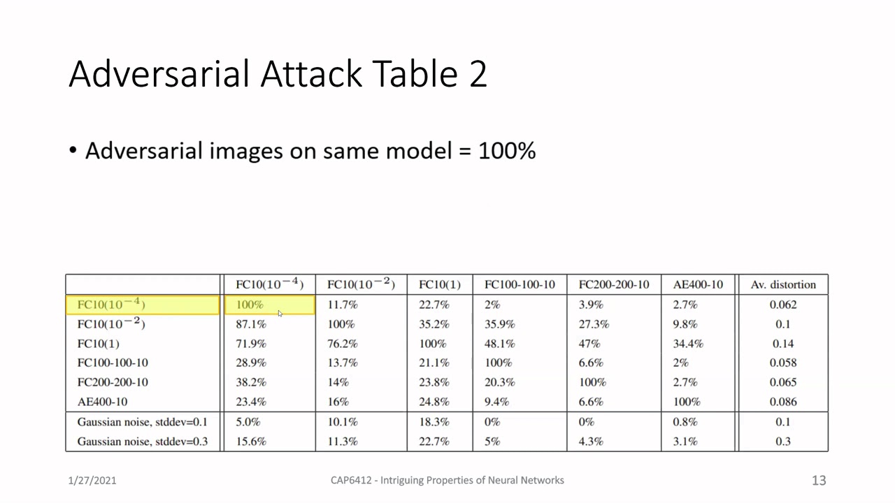
29:24
Intriguing Properties of Neural Networks Explained | CAP6412 Lecture Review
@UCFCRCV
1.1K views•2021-06-23

57:48
Secure Multiparty Computation (MPC): Foundations & Challenges
@SimonsInstitute
7.3K views•2015-05-28
64:01
Deep Reinforcement Learning Lecture: MDPs, Q-Learning, and Policy Gradients
@stanfordengineering
384.7K views•2017-08-11

18:41
Neural Networks Explained: Math, Layers, and Learning Fundamentals
@3blue1brown
21.9M views•2017-10-05
Related Study Plans & Knowledge Roadmaps
Structured learning paths in Artificial Intelligence
artificial-intelligence
Aligning LLMs: DPO, TRL & Custom Datasets
01Foundations of Python & Machine Learning
02Transformers and Large Language Models (LLMs)
03Aligning LLMs: SFT and RLHF
+ 3 more learning modules
24h6 modules
Explore Roadmap
artificial-intelligence
Federated Learning: PyTorch, Flower & Privacy
01Python & Machine Learning Foundations
02Deep Learning Basics with PyTorch
03Introduction to Federated Learning
+ 2 more learning modules
35h5 modules
Explore Roadmap
artificial-intelligence
Securing LLMs: Guardrails AI & NeMo Gateway
01Introduction to LLMs, Python, and APIs
02Understanding LLM Vulnerabilities & Threats
03Defending LLMs with Guardrails AI
+ 2 more learning modules
15h5 modules
Explore Roadmap
artificial-intelligence
Building Recommenders: Two-Tower & Vector DBs
01Foundations of Python & Machine Learning Basics
02Introduction to Recommender Systems
03Deep Learning & Representation Learning
+ 3 more learning modules
75h6 modules
Explore Roadmap