





![The moment we stopped understanding AI [AlexNet]](https://i.ytimg.com/vi_webp/UZDiGooFs54/maxresdefault.webp)

![[딥러닝의 기초] 251028 Chapter 6(2): Generalization, Regularization: theory and practice, Chapter 7(1)](https://i.ytimg.com/vi/CJqrEFeHxhk/maxresdefault.jpg)







![The Dangers of AI Adversarial Attacks: A PSA [Analog Horror]](https://i.ytimg.com/vi/LQZ_KOgt0aE/hqdefault.jpg)





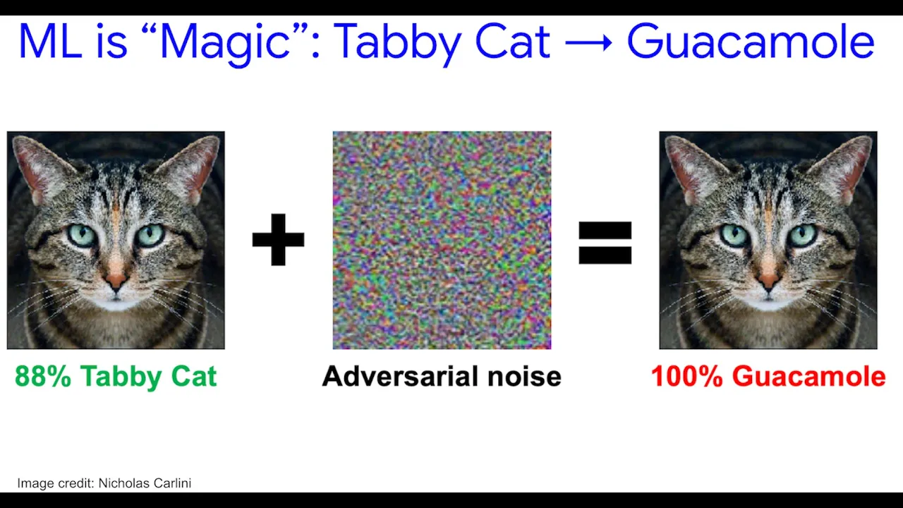
Neural networks exhibit two intriguing properties: (1) adversarial attacks can fool classifiers by adding carefully crafted noise, with these attacks being transferable across different models even when trained on different data subsets; (2) semantic information in neural networks is distributed across multiple units rather than being localized to individual neurons, challenging the assumption that individual units represent independent features.
Intriguing Properties of Neural Networks Explained | CAP6412 Lecture Review
Added:Fundamental concepts of Deep Neural Networks (DNNs), including backpropagation, loss functions, and gradient descent optimization.
An understanding of high-dimensional vector spaces and how neural networks learn latent feature representations.
The standard machine learning paradigm of generalization and the assumption of independent and identically distributed (i.i.d.) training and testing data.
Advanced adversarial attack algorithms such as the Fast Gradient Sign Method (FGSM), Projected Gradient Descent (PGD), and Carlini-Wagner (CW) attacks.
Adversarial defense methodologies, including adversarial training, defensive distillation, and certified robustness techniques.
The theoretical debate surrounding robust vs. non-robust features and how they contribute to model generalization.
Real-world security implications and vulnerability assessments of deep learning models in safety-critical domains like autonomous driving and medical diagnostics.
1.1K views17likes29:24Original Release: 2021-06-23
so today we will be discussing the paper um intriguing proper properties of neural networks uh james would be presenting for and i would be presenting against um so this is the presentation overview uh we'll look at some paper information the summary which includes the terminology used by the paper and the two intriguing properties one is which the adversarial attacks and the other one is the semantic information in units and then we look at the strengths of the paper weaknesses and maybe some discussion so the paper goes like this it was submitted in 2013 it was revised again in 2014 it's 10 pages long it's cited over six thousand times um although it looks intimidating uh it's not really that difficult so these are the authors uh these are fairly well known researchers uh doing active research and if you could see the citations 100k 200k so the terminology in the paper is slightly confusing they refer to unit which is actually a neuron it's a standard term in literature and the other one is the distortion in regards with the reversal perturbation distortion is measured by the standard deviation of the pixels which is uh the clean image minus that versus limit squared um summed over and then take an average this is the standard deviation so you are you are you are lowering down your sound yeah yeah so the first uh intriguing property is regarding the industrial attacks um until this point the assumption was that the classifiers are fairly generalizable and then they are fairly robust but the finding from this paper is that adversarial examples do exist adding carefully curated noise to the original images would actually alter the classification output of this neural networks and then the second um finding was that uh the semantic information in the units or neurons so the assumption was that the the neurons in the neural networks uh try to separate features try to learn independently different features but the finding from the paper is that this is not maybe true we look at each of these things carefully so for the adversarial attack they come up with this attack algorithm called lbfgs so if you try to recall dr shah has already touched upon this in the second lecture so it's a white box attack it's slow and it's a targeted attack so it goes on like this so there's a perturbation r we try to minimize the perturbation r such that when this r is added to a clean image x and then sent to the model f the output needs to be l is the class which is not the original label so we're trying to alter the label such that the perturbation is minimized also we need to make sure that the original image plus the perturbation lies in the range of the image which is bounds of the image which is 0 to 1 so this minimizer r might not be unique because we could have multiple such perturbations and then this makes this the problem really hard to simplify this the authors have come up with an approximation of this original problem by combining these two constraints whether try to minimize the c times r and the loss of the function um with the adversarial input and the label l such that um the distorted image still lies in the range of 0 to 1.
and this is optimized using the line search algorithm so this is the proposed adversarial attack algorithm and then this algorithm is used on various models and shown that investor examples do exist so for that they show this table if you could see the first column they consider six networks here the first three networks are fc10 and the value you see in the bracket is the lambda which is the weight decay parameter one of the hyper parameters for the model so they consider three different hyper parameters for fc 10 um and then a fairly complex model uh two complex models and then the auto encoder model so they consider six different models and try to attack these models with the proposed attack algorithm on the amnes data set so what they found out is that these adversarial examples do exist and they were able to achieve 100 fooling rate um on the mnist images so the final column shows here the minimum distortion um for each network required um to completely fool the network so other takeaway here is that the larger the lambda the larger the perturbations so the authors here here were trying to change the hyperparameter lambda to sort of include regularization in the network and to see um if they could still get the adversarial examples but increasing the lambda here as you see from 10 power minus 4 to 10 power minus 2 to 1 um has definitely increased the adverse average minimum distortion uh that is um making uh making the attack more difficult but on the other hand uh larger the lambda also means uh the accuracy is less on clean images so if you try to increase the lambda the test error keeps increasing so the training error and the test error here are on the clean images so at this point we are convinced that classifiers are not robust we we have succeeded in generating these adversarial examples so the next question here that arises is can we transfer these adversarial examples to a different model um say we have generated adversarial examples on one particular model and then try to send these adversarial examples to a different model do the transfer well this was the question and then to support this um they've given this nice table uh they've again considered the six models which we see on the first column um and then um each other column is for the same six models um to see how this cross model generalization of this adversarial samples work out so adversarial images on the same model uh turns out to be 100 um which we have already seen so we have 10 we have generated adversarial samples so it has a 100 full rate um on the same model so this is consistent across all models um so if you try to attack one model and send the same images again to the same model we get hundred percent full rate so now we try to see how um these adversarial samples try to behave uh when sent to a different models so consider the third model which is fc 10 we know that fc10 gives a 100 full rate when sent to the same model but what if we send to fc 10 then power minus 4 the first model so it gives out a full rate of 71.9 this means 71.9 percent of the time these adversarial samples were still valid which is quite interesting um so is this consistent across across all the models um maybe only sometimes let's see one more example the first model which is fc 10 10 power minus 4 when industrial samples was generated on this particular model um and then sent to the fourth model which is fc110 only two percent of the time uh it was able to transfer well all the other 98 percent of the time the model was able to predict correctly so at this point we can say that attacks transfer to different models uh but it's not always the case it's just sometimes and then if you see that these three models here are fairly complex and then when we try to transfer these models um the accuracy is low i mean the full rate is low so for fairly complex models the full red tends to be low and then just for the comparison they have given two rows in the end which is just random gaussian noise added to the images uh it's around five to ten percent which uh we can say that it's still much less than the these values which which are obtained by our optimization algorithm so rahul one one point here is that these models all these models were trained on the same data set right the same data so that's important distinction actually okay good yes all these are trained on mnist so at this point we can answer this question that sometimes these adversarial samples do transfer to different model but um but the question here is uh all these are trained on same mnist so obviously the the patterns and the learning thing would be the same for everything so what if we try to split the data set what if we uh train the models on different subsets of the data set that was the second question so if we could transfer to different model um and what if there's no training overlap what if these models are trained differently on different subsets of ms so this was the second question they try to address so for that they've come up with this experiment they come up with three different models here and these three different models are trained on different data sets the first model is trained on p1 uh p1 and p2 are two different subsets of mnist each having 30 000 images so the first data set here was trained on p1 the second sorry that the first model was trained on b1 the second model was trained also on p1 uh while the third model was trained on p2 so here we could observe that um sorry so here we could observe that when trained on p1 uh the error was zero percent so it was learning fairly well uh on the p1 clean image data set and then p2 when uh tested on p2 it's giving zero percent accuracy so it's learning really good but when uh it's when it's tested on the test set uh which is which is also a clean image data set um it's coming out to be two percent uh which is fairly a good network generalization we can say the first model is trained on p1 but when tested on the test set it gives a two percent error which means it's fairly generalizable and then the last column here is you see is the minimum average distortion so the minimum average distortion required to completely fool these networks so these are also similar so we can say that all these networks are consistent with these numbers so the next experiment here is that um we're trying to generate adversarial samples on one network and then try to test it on a different network so uh so what we see here is first these two models are trained on p1 as we have already seen and the third model is trained on p2 and similarly the columns the corresponding these two columns are regarding uh the models trained on p1 the third column is the model trained on p2 so what we see here is um so what we see here is how well do these adversarial samples transfer so for something uh so for the first model uh it's 100 when tested on the same model uh but when tried to transfer it from the first model to the third model it was just 5.9 percent again the first model was trained on p1 the third model was trained on p2 now we see a transferability of 5.9 percent and similarly for the third model when tested on p1 and the first and second models it's 8.2 percent so at this point we can say that um attacks do transfer to different models uh when there is no training overlap um but it's not maybe always the case um let's see the second uh part of the table so so the obtained uh adversarial samples are amplified um to see how well do they perform so when the amplified uh when they're amplified to standard deviation of 0.1 and then sent to the third model we see an increase in the uh fooling rate it's 43 and 22. and similarly for the third model it's 27 and 50.
so what we can say here is um so when the adversarial samples are right when they're amplified we see a higher full ratio and then when they are sending as in we see a slightly lesser ratio like five to eight percent so so rahul i have one question this yeah um so in the top one where you have cursor now so when you say when i look at the first row you say 100 yes so that is 100 is what is it the is it the fulling rate or is it what is 100 it's the full rate or the test error so as a 40 or the full rate is 100 percent full full-length 100 yes so so you generate these um adversarial example for this um first row and then you know they there then you taste it that it's successful and now when you do for the second column in the first row so it is uh much lower uh 26 percent but it still it works but when you go to third one which is a different partition right yes so then it's not that successful yeah it's not that successful so um so from here you know so so what's the can you repeat what's the conclusion from that first block of these three rows that it um yeah yeah the conclusion here is the adversarial samples do transfer to different models when there is no training overlap but to but but not to that great extent it's just five to eight percent so it's uh so this which means they are not effective that much effect not that effective yes yeah okay so that's the main point so i mean reasonable thing will be to locate the second column so they do 26 percent and which is okay but you know just five percent uh which is pretty bad okay good yeah continue yeah for the second question uh we can say sometimes it does sometimes it doesn't so it's fairly not that effective so the next question uh here is why how can these attacks exist why do these attacks even exist can we try to explain them using some mathematical formula so for that um the authors give this a really nice section 4.3 which is titled spectral analysis of unstability so let's say we have an input x and then the weight matrix w one um and then let let phi denote the output of uh some layer like five one demand the output of the first layer so when we try to send in the input image x with some parameters w1 the output would be phi 1 of x then this output is sent to the second layer which is the phi 2 of x and then so on so if the network has k layers um so the output of the neural network phi of x would be this particular thing so we try to um explain the unstability of this neural network the output of this neural network using the lip shifts constant so it goes on like this for some particular input image x and then for some particular perturbation we try to calculate the difference of the output um at some particular layer k in the neural network so we see that the difference in the output when given a clean image and then the perturbed image is always bounded by l times r l is the lipschitz constant i is the perturbation here and then when we try to generalize it for all the k layers here we get this really nice expression um uh the output of the neural network when sent into clean image which is phi of x minus the output of the neural network when sent perturbed image which is phi of x plus r is always bounded by l times the perturbation r here the lipstick's constant l is the product of all the lipsticks constants for each neural network layer and then to better understand the lipschitz constant it is just the largest slope if you try to see this picture here taken from wikipedia uh this purple line denotes the function f um and then we have uh x and the y axis um so the lipsticks um continuity so if some function is if it's lipschitz continuous uh we try to say that there's always a function there's always a constant l um which is which is which we can say that the slope of this function f is always bounded by this lipschitz constant l so if we try to move this r to this left hand side we get this difference in the response of the function divided by the difference in the input response which is basically the slope at point x and point x plus r which is always bounded by this constant l um so we get this really nice um cone sort of thing so talk about a positive negative before you go there yeah why there are two lines here yeah so the so the upper bound here is the positive l and then the lower bound would be the negative l and if we try to plot these two we get this two lines one is the positive l and the negative l and then when we try to run this uh over the function f we always see this see that this function always lies in this pink region it never goes into this cone so the so the l actually shows the slope of this cone so one is the positive l one is the negative value because we are taking the absolute value of yeah on the left side okay good yeah so after discussing this they come up with this uh table um so they try to develop a neural network they try to test it on mnist and then they try to calculate this lipschitz constant at each uh each layer so they see that for the first layer it's 2.75 for the second layer it's 10 third layer 7 so on so if you're trying to calculate the lipschitz constant for the complete network it would be the product of all these numbers so the takeaway here is that we see this instability is very early in this network so the first layer itself we see an upper bound of 2.75 the second takeaway is that this upper bound doesn't really prove the existence of adversarial examples it just proves that there are uh unstabilities in this network and then um but it doesn't really prove the existence of interstellar examples but what we can do here is we can try to reduce the upper bound uh we can try to reduce this upper bound which in turn reduces the instabilities in the network and then we can try to limit this attacks on the network yeah so for this question how can these attacks exist the authors try to explain it by giving this explanation by trying to formalize the network instabilities and then james would take over to discuss the other intriguing property yeah so we've covered the adversarial attack portion of the paper so the second portion of the paper discusses uh semantic information in the units the assumption was that units are separate features and the finding for this section of the paper was that maybe this isn't the case so this actually goes back to a couple papers published before this where the authors had analyzed individual units by finding the images in the data sets which maximizes that particular unit so they were analyzing a hidden unit by collecting the images the unit likes more formally it's denoted here where x is the input image e i is the natural basis phi is the layer activations for some arbitrary labor and then you take the dot product of that and then the images which maximize this are the images that the unit likes and in those papers that were published previously it appears to work quite well so here are a grouping of images and they all seem to have some similarities so in this case they all have they all are similar in that they'll have lower round strokes so those papers would describe that this unit is sensitive to those lower round strokes and likewise for imagenet these images all share the property of being similar to white flowers so describe that this unit is sensitive to white flowers however this paper challenges that by replacing the natural basis with a random vector so the only change is the vector that's getting multiplied so instead of only using one unit now you have a random combination of units and this also appears to work well so here is a grouping from the endness data set where all these images appear to have upper straight strokes or lower round strokes as soon as we describe that this direction instead of a unit so this direction is sensitive to those things and likewise for the imagenet um this direction appears to be sensitive to white and spread flowers to go over this in a more mathematical sense here we have two graphs and it's showing that the individual units aren't complete so they aren't on their own they aren't telling the whole story so red we have unit one in green we have unit two now looking only at one of those units we would get a local maxima so we get images that would be around this local maxima and same with the green unit however the more useful local maxima is the local maximum of the network which is a combination of those two units so the real feature would be following the black arrow and although it's possible to have this local maxima or the network local maxima align with the axis it's not likely because these spaces are really large so in conclusion for this section they got the same results for using single for maximizing single units versus multiple units and this suggests that the semantic information is spread among those units so it's not specific to a particular unit and they conclude that this method that other papers had used it was not a good method for analyzing these individual units so to summarize what this presentation has gone through this paper has concluded that the adversarial attacks question the robustness of these classification networks and that these attacks are transferable to different models and furthermore they're transferable to different models that haven't been trained on the same data set and then they give a mathematical basis for these attacks existing as well as a avenue of research for how to reduce the effect of these attacks and then the second part i concluded that the semantic information is spread among the units as opposed to individual units and it kind of concludes that analyzing the individual units is more difficult than the prior method would suggest so strengths for this paper i thought it had a really good explanations for higher level understanding uh specifically it related all of its conclusions uh back to core understandings of deep neural networks which helps to like more easily apply the knowledge you already have the experiment design for the second property with units was really simple and this helps make it really a really strong refutation of the method that previous authors had used and then the results for the attacks were very clear and they're very strong results especially for transferability and then there are widespread implications for these attacks in particular with transferability this vulnerability in classification networks wasn't known about and so for using classification networks for critical systems it's a it's a very important issue and then the mathematical analysis that they provided was really useful especially in creating a further avenue of research for trying to reduce the vulnerability of these classification networks and now rahul talked about the weaknesses okay and now for some weaknesses um so the two intriguing properties proposed uh seemed to be discharged to me uh i mean uh they didn't really connect these two properties well um i thought maybe they could have done it in two different papers with better experiments and then regarding the first intriguing property the random combination of units it's not well explained um how is this random combination of units uh taken is it uh totally random or is it a gaussian or a uniform distribution it's not very clear from the paper and the third one is the weak experiment supporting the first property this is regarding the semantic information among neurons they just give it one particular figure which shows which supports their claim but there is really no experiments for that adversarial input generation is not detailed the actual adversarial input generation the algorithm it's not it's not discussed in much detail it's just one section and then the results from that were still training are insignificant so once they got this adversarial samples they try to send in this back to the network along with the original cleaning images to see if it will learn better but these results seem to be insignificant it's just an improvement of 0.1 percent from the paper and then there's little evidence for extremely low probability of adversarial inputs so i've taken this line from the discussion section of their paper they say that this this adversarial inputs have this extremely low probability i don't see any evidence for this low probability of that visceral inputs uh so some thoughts uh so they say that um the the issue of this rugged decision boundary uh isn't quite addressed uh they try to do it by using this adversarial training but it doesn't seem to be very effective can we use the same optimization to retrieve the original label so right now we have added some perturbation we have changed the label uh can we again add some more perturbation in some negative way and then try to retrieve the original label back um using the same optimization method then the other one was uh if the number of classes is small will the problem be less severe there's also one thought and then yeah i feel this paper is really um thought-provoking and then it's a really good paper and then then we're open for questions and discussions
Up Next

10:08
Adversarial Attacks on AI Models Using FGSM | PyTorch
@EasyNextBytes
325 views•2025-02-15

57:48
Secure Multiparty Computation (MPC): Foundations & Challenges
@SimonsInstitute
7.3K views•2015-05-28

13:03
Bypassing Tor Censorship: Bridges and Pluggable Transport Guide
@Coding_ForEveryone
397 views•2024-06-11

18:41
Neural Networks Explained: Math, Layers, and Learning Fundamentals
@3blue1brown
21.9M views•2017-10-05
Related Study Plans & Knowledge Roadmaps
Structured learning paths in Artificial Intelligence
artificial-intelligence
Aligning LLMs: DPO, TRL & Custom Datasets
01Foundations of Python & Machine Learning
02Transformers and Large Language Models (LLMs)
03Aligning LLMs: SFT and RLHF
+ 3 more learning modules
24h6 modules
Explore Roadmap
artificial-intelligence
Federated Learning: PyTorch, Flower & Privacy
01Python & Machine Learning Foundations
02Deep Learning Basics with PyTorch
03Introduction to Federated Learning
+ 2 more learning modules
35h5 modules
Explore Roadmap
artificial-intelligence
Securing LLMs: Guardrails AI & NeMo Gateway
01Introduction to LLMs, Python, and APIs
02Understanding LLM Vulnerabilities & Threats
03Defending LLMs with Guardrails AI
+ 2 more learning modules
15h5 modules
Explore Roadmap
artificial-intelligence
Building Recommenders: Two-Tower & Vector DBs
01Foundations of Python & Machine Learning Basics
02Introduction to Recommender Systems
03Deep Learning & Representation Learning
+ 3 more learning modules
75h6 modules
Explore Roadmap