



![[INFO257] Unidad 4 - Tutorial de Pytorch 2](https://i.ytimg.com/vi/fji4vRiyMZ8/maxresdefault.jpg)





















The Fast Gradient Sign Method (FGSM) is a white box adversarial attack technique that exploits how AI models learn by adjusting input data rather than model weights to maximize loss, using the formula: perturbed_image = original_image + epsilon × sign(data_gradient), where epsilon controls the perturbation magnitude; this attack can cause models to misclassify images with high confidence even when perturbations are imperceptible to humans, as demonstrated by an example where a panda image was misclassified as a gibbon with 99% confidence after adding a small perturbation.
Adversarial Attacks on AI Models Using FGSM | PyTorch
Added:Understanding of Convolutional Neural Networks (CNNs) and how they process image data for classification.
Familiarity with the PyTorch framework, specifically tensor manipulation, loading pre-trained models, and executing a forward pass.
Fundamental knowledge of loss functions (such as Cross-Entropy Loss) and how backpropagation computes gradients.
The core concept of gradient-based optimization, particularly understanding how gradients indicate the direction of steepest ascent or descent.
Adversarial Training: Learning how to train neural networks on adversarial examples to build robust, defensive models.
Advanced Iterative Attacks: Exploring more sophisticated threat models like Projected Gradient Descent (PGD) and the Carlini & Wagner (C&W) attack.
Black-Box Attacks and Transferability: Studying how adversarial perturbations generated on a surrogate model can successfully fool a target model with unknown architecture.
Robustness Evaluation Frameworks: Utilizing specialized security libraries such as Foolbox, CleverHans, or Adversarial Robustness Toolbox (ART) to benchmark model vulnerability.
325 views5likes10:08Original Release: 2025-02-15
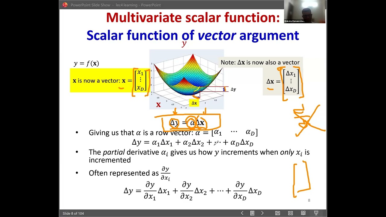
hi in this video we'll look at how to attack an AI model generally AI models are trained using data and they perform well after the training has stabilized the concept of advis attack is that an adversary is interested in modifying the neural network such that it generates wrong outputs in many cases these take the form of imperceptible perations that are added to an image and cause the network to generate misclassified outputs two common forms of attack vectors are white box attacks and blackbox attacks white box attack model assumes that the attacker has full knowledge and access to the model whereas blackbox attack assumes that the attacker only has access to the inputs and outputs of the model but not the internals of the model fgsm or first gradient sign attack is a white box attack model as we saw in one of the previous videos the way AI model learns is by adjusting the model weights to minimize the loss based on the back propagated gradients the fgsm attack model similarly adjusts the input data rather than the model weights to maximize the loss rather than minimizing it based on the back propagated gradients more detail about this model is available in this paper let's look at an example output of such an attack on the left we see in the image of a panda and to this image if we add an imperceptible perturbation as shown by this image in the middle and we scale it by an Epsilon value of 01 and we add this image pixel wise to this image we get the output result on the right hand side when the image on the right hand side is sent to the same neural network that was originally trained to classify this left image as a panda it turns out that the model thinks that the image on the right is a given and not a Panda and also the model is overly confident that it's a gibbon so the confidence has increased from 57% being Panda to 99% it being a given so let's see how we can generate an attack of such form we do our usual Imports on the input side we have a set of Epsilon values these are the scaling factors that are used to scale the amount of pertubation added to the input image we use a pre-trained model from the linet Network that has been trained on the mes data set then we recreate our model class this model consists of two convolutional layers two Dropout layers and two fully connected layers the forward function of this class takes in an input X passes it through all the individual layers and generates the output in in terms of test data we use a test loader which is a data loader and pass it to the mest data set and we apply two transforms to the data first we convert each input sample to a tensor and we also normalize the tensor using the mean and standard deviation values given here as an example if you get the first example from this test loader we see that it generates two outputs X and Y X is the image which is of shape 1 by 1 by 28 by 28 where in the first one is the batch the second one is the channel number of channels being one and then 28 x28 is the number of pixels in the mnus data set for each image why is the corresponding label for this first example we choose the device ideally you would have a machine with the GPU but in this case I have a machine with a CPU so the training will be slower first we initialize the model given by the model definition above we pass it to the device we load the state dictionary from the pre-train model weights that we had set the path to previously we map it to the device then we set the model to evaluation mode focusing on the fgsm attack the attack function needs three inputs first is the clean image that we want to perturb Second Epsilon is the pixel wise pertubation amount or the scaling factor that we need to apply and third is the data gradient or the gradient of the loss with respect to the input that can be seen here where we are Computing the gradient with respect to X which is the input of the loss function J where J is a function of the network parameters Theta the output of this function is a perturbed image which is essentially the summation of the image along with Epsilon times the sign of the data gradient so in code it looks like this we take the sign of the gradient we take in the Epsilon value that was passed in multiply it by the sign of the gradient add it to the image and out comes the perturbed image and then we clamp the perturbed image in the 0 to one range and return it we also need a denormalization function which removes the normalization that was applied as part of the transform the data loader in the test function for each sample in the test set we compute the gradient of the law with respect to the input data which is data Grant we create the perturbed image by calling the fgsm attack function which gives us perturbed data and then we check if the perturbed example is adversarial or not which means that whether it has been misclassified or not looking into the test function in detail we Loop over the X and Y from the data loader in this case it's a test loader so we have each image stored in data and the corresponding label stored in Target we move the image and Target to the device we set request grad equals to true so that we compute the gradient with respect to the input we generate the output of the model on this data by doing the forward pass we get the initial index of the predicted label for that data if the initial prediction does not match the target prediction which implies it's already a misclassification so we don't bother attacking it further otherwise we compute the loss zero out all existing gradients calculate the gradient of the model in the backward pass and then store the gradient of the input in the data grad variable we then do the denormalization of the data and then call the fgsm attack function by passing in this denormalized data the Epsilon scale SC in value and the data grad which is the gradient of the loss function with respect to the input what we get out is the perturb data which is the modified image or the modified data after it has been attacked using the fgsm attack function we then reapply the normalization by calling the transform.
normalized with the same mean and standard deviation values and then reclassify this perturb data by passing it through the model and generating the new output and then we check for success by looking for whether the predicted output matches the target output or not if it does not match then it implies that the advis attack has been successful and we store few advis examples to view later on we calculate the accuracy using this Epsilon value over all the samples and then we return the final accuracy and the sample set of advisal examples finally we call the test function by running the attack on the different values of Epsilon and for each Epsilon we get back the accuracy and the set of adversarial examples which we store in a list of accuracies and examples next we plot the accuracy of the model against these different Epsilon values what this graph shows us is the accuracy versus Epsilon plot this indicates that as the amount of Epsilon increases which is the amount of perturbation that has been added which is a scaling Factor the accuracy of the model decreases as we would expect it to be one thing to note is that the decrease in accuracy is not linear as in it does not decrease by the same slope as we increase the Epsilon but there is a strong nonlinearity behavior in the decrease in accuracy so somewhere the model reaches the accuracy of 0.1 which is the same as a random guess for 10 classes next we look at some of the advisal examples that have been generated and plot them in a figure each row here corresponds to different Epsilon values where Epsilon equals to Z implies no perturbation has been applied which is why the predicted label matches the target label as we keep increasing the Epsilon we can see that there are small amount of perturbations that have been added to the input and if we look at this example the true label of this image is three but after perturbation the image has been misclassified as label two similarly for this example the original image label is four but after perturbation it has been misclassified as nine as you can see as we increase the Epsilon values the amount of noise keeps increasing in the image and it's no longer imperceptible and at large Epsilon values the noise starts becoming extremely powerful and visible in the image this is one form attack the fgsm attack there are other ways to attack the models and generate adversarial outputs that's it for this video see you in the next one
Up Next

85:00
Trustworthy ML Lecture 4: OOD Generalization & Adversarial Attacks
@TübingenMachineLearning
904 views•2023-11-06

57:48
Secure Multiparty Computation (MPC): Foundations & Challenges
@SimonsInstitute
7.3K views•2015-05-28

13:03
Bypassing Tor Censorship: Bridges and Pluggable Transport Guide
@Coding_ForEveryone
397 views•2024-06-11

18:41
Neural Networks Explained: Math, Layers, and Learning Fundamentals
@3blue1brown
21.9M views•2017-10-05
Related Study Plans & Knowledge Roadmaps
Structured learning paths in Artificial Intelligence
artificial-intelligence
Aligning LLMs: DPO, TRL & Custom Datasets
01Foundations of Python & Machine Learning
02Transformers and Large Language Models (LLMs)
03Aligning LLMs: SFT and RLHF
+ 3 more learning modules
24h6 modules
Explore Roadmap
artificial-intelligence
Federated Learning: PyTorch, Flower & Privacy
01Python & Machine Learning Foundations
02Deep Learning Basics with PyTorch
03Introduction to Federated Learning
+ 2 more learning modules
35h5 modules
Explore Roadmap
artificial-intelligence
Securing LLMs: Guardrails AI & NeMo Gateway
01Introduction to LLMs, Python, and APIs
02Understanding LLM Vulnerabilities & Threats
03Defending LLMs with Guardrails AI
+ 2 more learning modules
15h5 modules
Explore Roadmap
artificial-intelligence
Building Recommenders: Two-Tower & Vector DBs
01Foundations of Python & Machine Learning Basics
02Introduction to Recommender Systems
03Deep Learning & Representation Learning
+ 3 more learning modules
75h6 modules
Explore Roadmap