![[Easy! 딥러닝] 4-1강. Validation 데이터가 꼭 필요한 이유 | 테스트 데이터와 차이점은??](https://i.ytimg.com/vi_webp/6daz8eH22sA/maxresdefault.webp)





![#34 Machine Learning Specialization [Course 1, Week 3, Lesson 2]](https://i.ytimg.com/vi/vq4Ie5xWhww/maxresdefault.jpg)



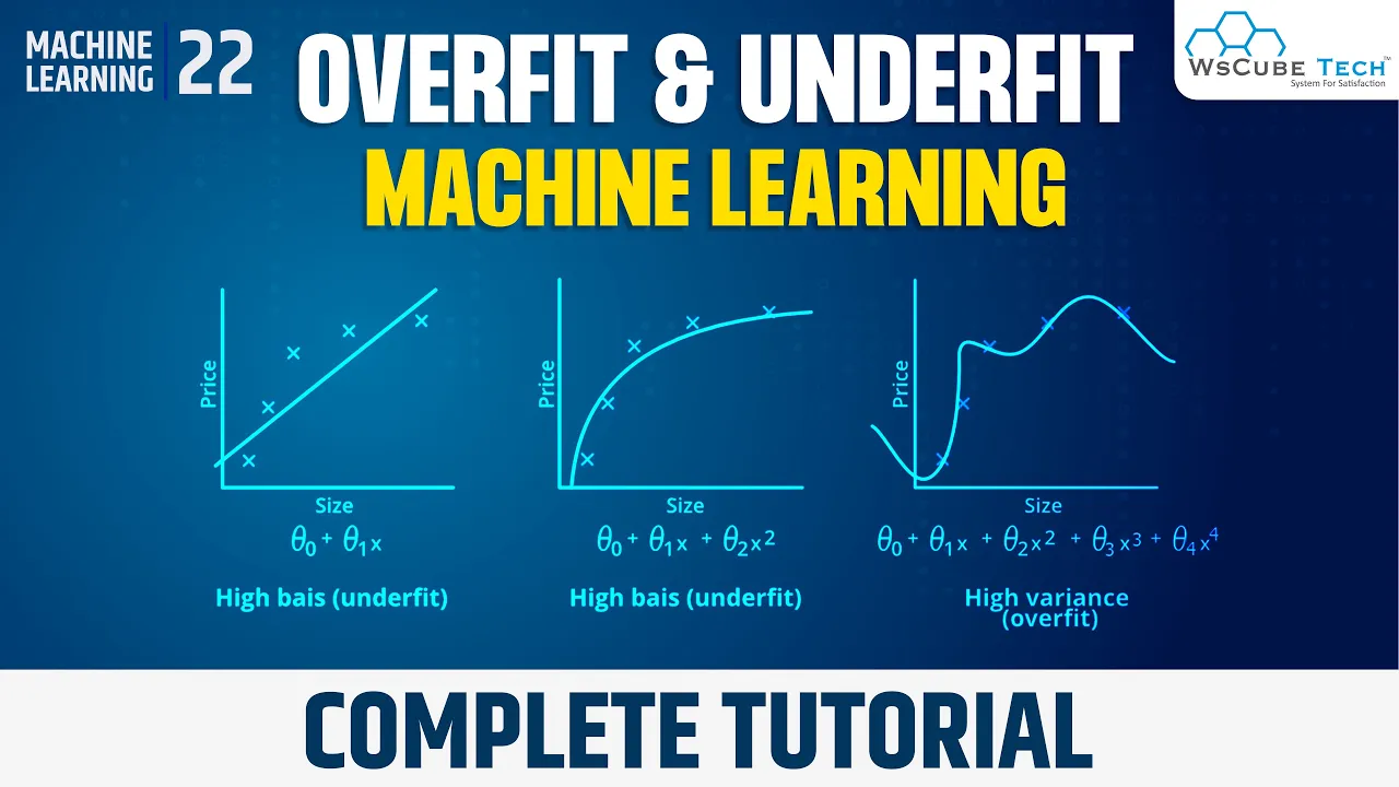
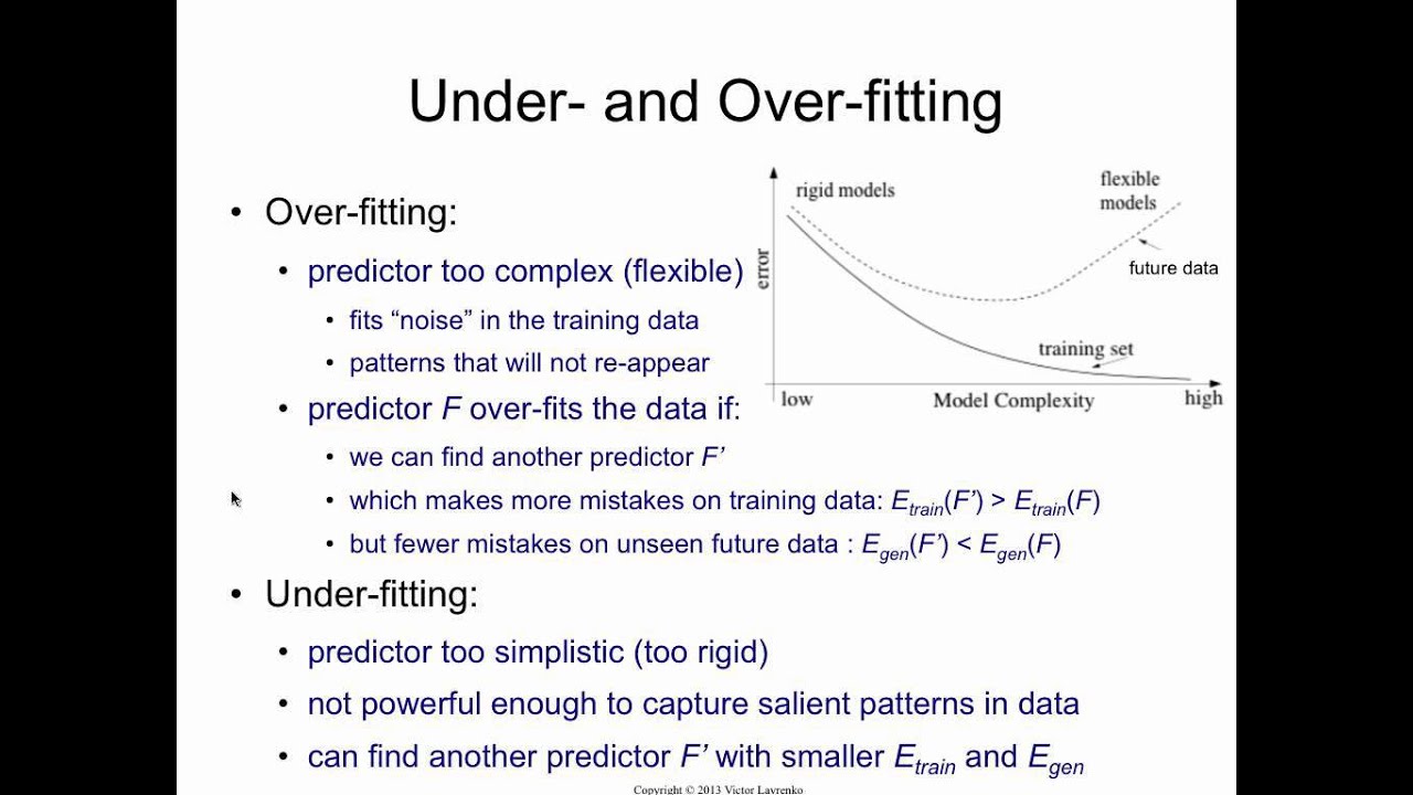




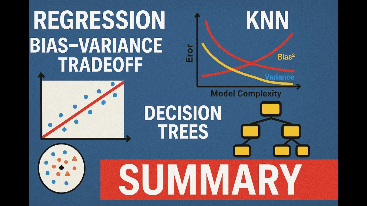





In machine learning, the bias-variance trade-off describes how model complexity affects generalization error: high bias (underfitting) occurs when models are too simple to capture true patterns, while high variance (overfitting) occurs when models are too complex and fit training noise; generalization error can be decomposed into irreducible error (data noise), bias squared (model expressivity limitations), and variance (finite sample sensitivity), and regularization techniques like L2/L1 penalties help balance this trade-off by penalizing large parameter values to encourage smoother, more generalizable hypotheses.
Stanford CS229: Bias-Variance Tradeoff, Cross-Validation & Regularization | Lecture 12
Added:Familiarity with supervised learning fundamentals, including the conceptual difference between training, validation, and test datasets.
A solid understanding of linear and logistic regression models, including how they are optimized using cost/loss functions.
Basic probability and statistics concepts, specifically expected value, variance, and probability distributions, which are essential for deriving the bias-variance decomposition.
An intuitive grasp of underfitting and overfitting in predictive modeling.
Exploring Statistical Learning Theory, including VC (Vapnik-Chervonenkis) dimension, Rademacher complexity, and generalization bounds.
Advanced mathematical derivations of regularization techniques, such as L1 (Lasso) and L2 (Ridge) regression, and their Bayesian interpretations (MAP estimation).
Ensemble learning methods, such as Bagging (to reduce variance) and Boosting (to reduce bias), to see how these trade-offs are managed in practice.
Implementing automated hyperparameter optimization techniques (e.g., Bayesian Optimization or Grid Search) using cross-validation as the evaluation metric.
20.6K views183likes1:55:40Original Release: 2021-04-20
okay welcome back everyone to lecture 12 of cs229 the topics for today are bias variance trade-off model selection and cross validation and regularization the three are are kind of somewhat related to each other and i would say bias variance trade off is probably one of the most important topics that you need to take away from this course it it it's at the heart of machine learning and the concept that kind of is unique to machine learning and distinguishes it from other fields right so a quick recap of what we covered uh over the last two classes so the last two classes we covered neural networks and deep learning and the the main takeaways from the last uh two classes was the neural networks are basically composition of simple building blocks where the simple building blocks are you know linear models that we've seen in the past so we we we take the output of one one simple model and feed that as input to you know another simple model and so on and the crucial crucial thing while composing the composing them is having non-linearities right and non-linearities are crucial because if there were no non-linearities then the entire network could be represented as just a single linear single linear layer with one one matrix and also neural networks and deep learning they are they are non-convex and it's important that we initialize the parameters randomly whereas in the previous models that we saw the simpler models they were mostly convex and initialization did not matter but for neural networks for example initializing all your parameters to 0 will not work because because of the symmetry symmetry properties that we that we discuss and then the approach for training neural networks was basically back propagation back propagation is just a fancy name for the chain rule of multivariate calculus and what we saw was we calculate the gradients of the final loss with respect to every parameter at all layers and in order to calculate those those gradients we use the multivariate chain rule so the last layer was you know a linear uh a linear model that we've uh you know very similar to glms and then from from beyond the last layer as we as we compute the gradients of parameters from earlier layers we see we saw that you we encounter a chain of very simple jacobians they are either diagonal jacobians where each diagonal entry is the derivative of the non-linearity or it's going to be the weight matrix so the weight matrix itself will be the jacobian right and [Music] we we construct the simple chain of jacobians until we arrive at the layer at which we are calculating the gradient from and then from from the the branch that's specific to that layer it was pretty pretty straightforward calculus that the notation was a little heavy but it's it's pretty much you know there's nothing nothing fancy going on there it's just simple simple uh gradients that we need to uh that we need to take and to the end of of uh the last lecture we saw this um or we just discussed this theorem which is you know it's not going to be in your in your syllabus and we're not going to test you on that theorem uh but it's a it's a good kind of segue into bias variance because the universal approximation theorem suggests that neural networks can be very expressive so it can represent any possible any any smooth and differentiable function on a given input range and that that kind of ah brings us into bias variance and asking the question is that a good thing or a bad thing you know having having expressive models is that is that good or is that bad so that brings us to bias variance any questions on neural networks or deep learning before we jump into uh bias variance any remaining questions okay so uh bias variant so in in your homework one in in the last question where we we saw feature maps right so in feature maps we ah supposing we had a data data set that looked like this i'm plotting the same data set again here and here it's the same data set right now if we fit a linear model where the feature map is just a polynomial of degree 1.
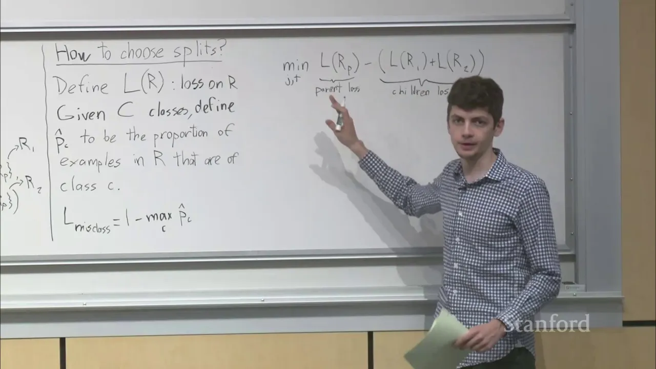
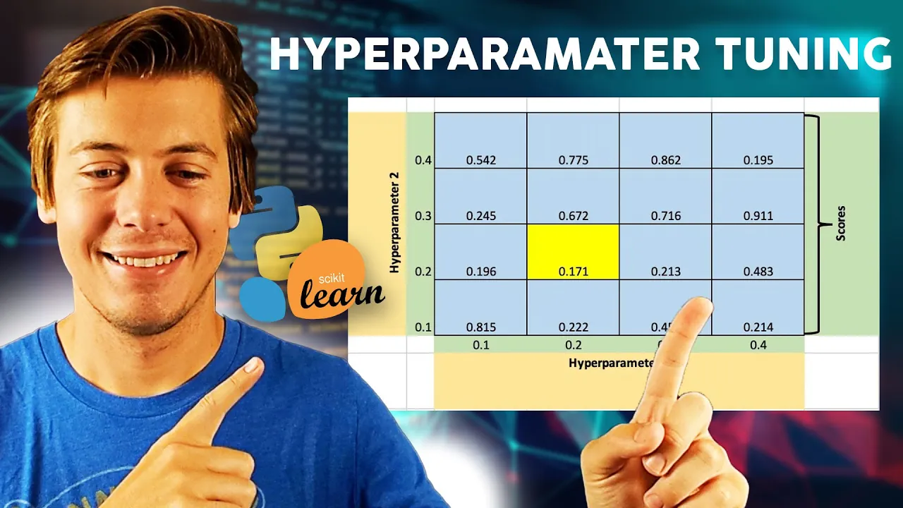
so k equals 1 we get a straight line fit through the data and if we try with k equals 2 whether the polynomial degree is 2 we get say a quadratic fit similarly if we try with say k equals 20 right we would get a fit that might look something like this right now we could have done something very similar with say a classification problem right supposing the x is here mark one class and o's mark another let's say this one x here and one over here supposing we had a data set like this and say third i am just copying the same data set in three different places here the ah x's mark one class and the o's mark another class now if we try to fit say a logistic regression with polynomial features say with k equals one we would again get a straight line fit that tries to separate the two classes if we try the logistic regression with k equals two we would get a quadratic fit and let us say we tried it with k equals you know maybe twenty right and we we would probably get something that could potentially look like this right so um loosely speaking we can call these models as being underfit these models as overfit so in machine learning we are given a training set but the the the error that we actually care about is not how well the model performs on the given data set but how well does the model perform in general on data that it has not seen before you can call it loosely speaking the test set but in general you know you you call it generalization error so generalization error generalization error is the error or the loss or the cost that our model incurs when it is tested against possibly all the infinite data out there in the world from whose distribution we got the training set right and in machine learning what we care about is that our model needs to have a low generalization error but the the fundamental problem is that what we have access to is just a finite sample from the from the you know uh the the uh infinitely many possible examples from the uh data distribution we have a finite sample from the data generating distribution and we need using this finite sample we need to build a model that has good error rate or low error when it is tested against all the possible you know infinitely many examples in our data distribution so this this concept of under fitting and over fitting is you can you can think of underfitting and over fitting as corresponding to different uh components of the generalization error so loosely speaking generalization error which means taking the model that we obtained and testing it against an example that we have not seen before and when we test it against an example that we've not seen it before there is going to be some error it's never going to be perfectly right and that error can be broken down into sub components right so the generalization error can be broken down into two parts a component called the bias and the component called the variance and loosely speaking ah bias is the component due to what you can call as this is the component of generalization error i am going to write it as g e component of this generalized error due to expressivity handicap and variance is the component of generalization error due to finite sample of training set right and the generalization error that is incurred by this model you expect it to be pretty high and the generalization error incurred by this model is also expected to be pretty high but they are high for fundamentally very different reasons the reason why this model or these kinds of models are expected to high have high generalization error is because they are linear models and they are kind of have handicapped and cannot capture this quadratic relation between between the x's and y's similarly this model is extremely expressive it can twist and turn in wild ways but it it it cannot generalize well because it just it does not have enough enough data to kind of ah fit it fit it well rather so it does extremely well on the given training set and in order to do well on the given training set you know we are kind of you know losing the big picture of wanting to generalize well on unseen data and we do overly well on the training side right and this is due to the fact that we just don't have enough training data right if if we had a lot more number of training data then even though we had a higher expressive model it wouldn't have overfit on the data like this right and and we saw some amount of that in your homework question as well where if uh if we start with a small data set where the number of examples is very small then the higher order polynomials can over fit it by you know by forming highly wiggly hypothesis functions whereas if you had a larger data set even polynomials of higher degree can you know do a pretty good job of fitting the data so loosely speaking bias is the generalization error of a model due to it being kind of handicapped in its expressivity and it just cannot uh even do a good job of fitting the training set itself very well and variance is is uh is due to the fact that your model was highly expressive but it just did not have enough data for for it to um for it to generalize well right and these concepts um these definitions are very loose these are not standard definitions but this is a good good kind of intuition to have of of what bias and variants are in fact when we are using the squared error as the loss function in the setting of the squared error and where the model is and we assume that our data comes like this y equals f of x plus epsilon where f is some function you know some hypothesis right um if if this is the true data generating distribution where the expectation of epsilon is 0 and the variance of epsilon is sigma square right for in in this particular setting the generalization error or the test error which is also the generalization error is equal to you know the expected y minus f hat x square now lets lets analyze this for a moment so f hat let me suffix it with n f hat n is the is the model that we get by fitting on n training examples right and the n training examples were obtained with this data generating process which means the n training examples now are obtained with y i equals f of x i plus epsilon i right so the n training examples from which the f hat was ah obtained had noise embedded in them right and therefore f hat n is a random variable it is a random function it is a random variable because it is a function over inputs that were random right so f hat n is it accepts an input as x x is not random but the way f hat n was constructed was using n training examples and the n training examples had noise in them and therefore because the n training examples had noise in them f hat n is random it is random but it accepts an input which is deterministic but the way f hat n itself was constructed was is it's a random variable and what is this expression um what's this expression calculating it is calculating over here x and y are appear from the test test set or on on an example that the model has not seen before so on an example that the model has not seen before what is the prediction of our learned model on the new input and this is the error of of that model with the new output right so this is generalization error and this expectation is over the noise that is in the test example and noise in the training set right so this is the expectation over all the noise uh noise uh variables both in the training set and the test set right so where expectation is over all epsilon in training set and test example right and in the case of the squared error we can see that this can be with some pretty simple pretty simple algebra we can show that this will be equal to sigma square plus expectation of f of x minus f hat x square plus variance of ok so over here f is the true function that we do not have access to and f hat f hat n is the model that we obtained by training on the finite training training data and we can decompose this this error on a new test example as into three components right this component is called irreducible error and this component is called the bias squared bias squared and this component is called the variance right so what is happening here so what what this is telling us is the test error of any model can be broken down into into these three components now all of these three components are non negative because this is this is a sigma square that is the variance of the noise that is non-negative this is the bias squared so that is non-negative and this is the variance of something and that is non-negative so the test error or the expected test error can be broken down into three components now each of these each of these three errors is a is a fundamentally very different kind of error compared to the other two so irreducible error tells us that no matter what kind of model we choose no matter how big training how big a training set we start with we can never do better than irreducible error and why is that that's because fundamentally data is noisy which means for the same given value of x for different examples y can be different because of the noise term which means at test time when we are given a value of x on which we need to make a prediction the y value could be multiple possible y values and there's just no way we can we can ah you know get the right get the right prediction all the time because our function f is a deterministic function right and that noise is essentially what's captured in this irreducible error right so irreducible error is because the data is noisy and for given value of x there is no single right answer right that's irreducible no matter what kind of model you choose you choose a neural network you choose a linear regression choose any fancy model you want you can never do better than irreducible error any questions on this yes minus the actual so the question was uh why is this irreducible error because by increasing k we we actually made it go through all the points so um and and the question is you know is an epsilon zero in this case uh the the uh answer to that is here we are talking about test error which means now we are measuring how well this model performs on a test point that was not included in the training set right so this is generalization error which means we are measuring how well the model performs on unseen data right because doing well on the given training set is an easy thing right there you know it's there is you know you don't need so much of theory to do well on just the given training set that you have in fact if you're just given a training set and you want to do well on the training set just memorize the training set right the whole point of machine learning is to start with a limited set of training data and still do well on generalization error right so generalization error is when you are given a new example that we have never seen before the expected error can be decomposed into an irreducible error component which is due to the fact that the data is noisy and then there are two more components here now what are these two components so the first one is the expectation of f x minus f hat n x so what does this mean there is a true underlying signal that we do not have access to and the true underlying signal will be different from the prediction made by our model and in general what is the expectation of this of this ah of the difference between of or the difference between the true underlying signal and our uh and the prediction that our model makes in general and if we take the expectation across all the all the possible different training sets that we get and expectation across the noise in the test example that gives us how how systematically wrong are we right what is the expected expected difference between the true signal and um and and the predicted uh predicted value and this is the square of that bias and finally we have uh a third part called the the variance of f hat and x now what is what is the meaning of the variance of f hat and x it means if we were to repeat this experiment with a new set of n examples right i do not mean repeat the experiment of refitting on the same data set repeat this experiment by collecting a new set of n examples from the same data generating distribution f hat nx will be a different the prediction on the test set will be a different value right and now if we were to keep repeating this process over and over by collecting a new set of an examples and making a prediction on this uh test set you know and repeat again a new set of n examples fit the model make a prediction on uh the new test set x all these different predictions on the new test set is going to have some variance in it right and this is the variance of the prediction made on a new test example when we are changing the training set to be a resample every time right and this variance you can kind of see was completely unrelated to what the right answer for f for the new test example was right it's just how how sensitive to noise we are in the for the noise in the training set and and that's captured by variance this question right so the question is uh because we said variance is is due to the limitation of having a finite sample test set now you can imagine um if your population has you know theoretically it has an infinite number of number of ah points infinite number of examples if you were to take the entire infinite set of training population and fit your model and would you were to repeat it by taking the entire infinite set again and fit your model you always get the same model right and the the variance that we get from experiment to experiment where the experiment includes collecting your end training examples the the the variance that you get from experiment experiment is due to the fact that you're collecting a small number of finite examples if you were to collect more number of examples in each experiment then the variance will come down and we'll go a little bit deeper into this shortly so coming back to your question about the polynomial case um in in our homework uh question five what we saw was with uh k equals 20 it was a pretty uh wiggly function now if we were to repeat the k equals 20 case with a data set of say 10 000 examples then what you will see is that it it will do you know fairly well it will fit it fairly well you re-sample a new set of what was the number of said twenty thousand or whatever you know ten thousand examples you repeat it it will be slightly different right and you repeat it again you'll get a new hypothesis which is again very slightly different and if you were to repeat this experiment with a new number say you know 10 million examples then the the the variance from experiment to experiment is going to come down even further right the more number of examples you have they may be noisy right you know you take 10 000 examples each of those examples has noise in them but the variance in the fitted model from experiment to experiment is going to come down the more number of examples you have we will come to that so the question is you know is it uh is the relation linear or quadratic we will come to that shortly right so this is in the context of machine learning right however um however i think understanding bias and variance from a more classical statistic statistics setting is a little more intuitive than understanding this so so let us have a look at bias variance from a more classical statistics setting because here we were focused on prediction now how well does the model or what does the model do when it is presented with an x that is it has not seen before right so bias variance in a more um so lets assume there is a data generating distribution ah data x comma y our pairs come from some some distribution that's parameterized by theta right and what we do is from this data generating distribution we collect n examples so each of this is a pair x1 y1 until xn yn right we we sample x and y pairs from the data generating distribution and we sample n such insert pairs and we run it through a statistical model right and by a statistical model ah what what i mean is say the mle estimator you know it and what we get out is a theta hat right this is what we did for example in in linear regression you know if if we assume a linear relation between x and y where the theta captures the linear coefficients then this is just the normal equation right but in general it is some some statistical model if if this is you know x is x is some features and y is 0 1 then you know think of this as logistic regression and once you once you fit the model you get the the estimated parameters right so now this is random random because they were random samples from our data generating distribution right and this is not random this is you know deterministic right and what happens when you feed a random variable into a deterministic function the output will be random right so this is also random and the weight is random ah we can we can visualize so let us assume we have four different statistical models right so this is theta one this is theta d theta d and this is our parameter space you know one so over here we were looking at the data space right so here this was x and this was y and here this was x1 and this was xd right over here we are in the parameter space right that's that's uh so it's a switch from that view theta one theta d theta one and theta d now the the the data that we sampled from came from some true distribution let us call it theta star right so theta star is some unknown unknown constant that you know we do not have access to so let us you know assume theta star was here this is theta star drawing it in the same position in all the four theta star this is theta star yeah so so this this is basically in the same position in all the four ah four and let's let's assume we have four different statistical models four different estimators of our parameter right and we start an experiment we sample n examples from this distribution here we are assuming we have access to you know potentially sampling an infinite number of points and assume sampling is cheap right sample n examples where n is some fixed number run it through this statistical model run it through each of the four models so we have so let us call this model a model b model c and model d and these four plots correspond to a b c and d right and for a given sample of ah n examples we get some estimate theta hat right so maybe you know this was the estimate by a and by b maybe this was the estimate right and maybe from c this was the estimate and maybe from d maybe this was the estimate right so unfortunately i do not have colored pens here but maybe i will highlight this with with a the true parameter make it a little bigger as a block because i do not have a different color pen today right and and supposing we repeat the experiment get a new set of n examples fit it on the four different models and because the new set of examples had you know noise in them the estimated theta is going to be different again right and in this case let's say the new estimate was here and in this case the new estimate let's say was was here and over in this case let's say it was here in this case let us say it was here right and then we repeat it set of n run it fit it through four different models and plot the estimated values right so let's say it was here and let's say we keep repeating it so each each dot in these plots corresponds to one experiment right it is the output of one experiment right the number of dots is not the same as the number of examples so the number of each dot corresponds to one experiment and what we see is um we might get plots like these and what we would call what we see here is in in these in these two examples the the variance of the expected the variance of the estimator is pretty small because they are they are you know because they are pretty tightly concentrated in one region right whereas in these two cases the variance is pretty large right so you would call these two as low variance and these two as high variance so a low variance estimator and high variance estimator right and similarly what we see is over here the distribution of theta hat so you can you can think of the dots that we obtained by you know repeating this process as samples from theta hat the distribution of theta hat and that's also called the sampling distribution right so these each of these dots are samples from the corresponding sampling distributions right and what we see is the sampling distribution is kind of centered on the true value right so so the center of the sampling distribution coincides with the true value in both the cases right so this is so this is therefore called a low bias estimator and this the center of the sampling distribution is has moved away from the true parameter so these you would call them as high variance estimate high bias estimators so what we see is that bias and variance are are fundamentally different things right having one each having having low variance or high variance says nothing about whether the model has high high bias or low bias the way to think about high bias is that the estimator has has a fundamental systematic error in estimating parameters in that no matter how many times you you sample different data sets and fit them in this case they are you know fundamentally kind of there is a systematic bias say in this case to be closer to zero right and that has got nothing to do with whether they have low variance or high variance similarly this model has low variance these these these models have low variance which means no matter uh no matter how much noise no matter the noise that you get from you know different uh training sets the estimated value is somewhat you know tightly tightly grouped in some region right so the the um it is less swayed by the noise in the training set that's one way to think of it right in this case it may have a systematic error in this case it may not have a systematic error but the these estimators are less swayed by the noise in the training set whereas these these two models are pretty sw they are sensitive to noise in in the training set so um depending on the specific set of n examples you know the the variance in the estimated values are pretty large any questions on this yes yeah so i'll come to the trade off why we call it a trade-off what we what we then notice is instead of n examples let us say we collect a much larger set of say capital n you know which is a much larger training cycle say thousand times the size right so x 1 y 1 all the way till x capital n y capital n if you increase your data set by a large fraction by a large amount what we observe is that in all the four cases the variance will come down right so so with a large larger data set so this is a b c d let's say these were the true values yes so instead of small n number of samples we are repeating this this cycle of experiments with capital n examples in each experiment what we see is that the variance is going to come down and in this case right so this is with n examples and this was with small n examples right so what we see is that this is still has some bias left but the variance has reduced much more right and in this case in all the cases the variance has come down right but the the these two still remain unbiased these two still remain biased and as n is increasing we see that the bias is also kind of reducing as n increased from here to here and thats a pretty excuse me thats a pretty common phenomenon as well as you increase as you increase n your your variance will almost always come down and the bias also generally also comes down so so in a classical statistical setting the expected difference between theta hat so the expectation of theta hat is going to be the the center of your sampling distribution right so in in in classical statistical setting the expectation of theta hat minus theta star is called the bias if the the mean of the sampling distribution is centered exactly at theta star then the bias will be zero right and the variance of theta hat is called the variance right and if the as n tends to infinity so if the bias tends to zero as n tends to infinity then this is called a consistent estimator right so what does it mean as as as the number of examples goes to uh goes to infinity the variance you know will generally come down but also if the bias also goes to zero as n tends to infinity then it is called a consistent estimator for example [Music] in in case of gaussians the maximum likelihood estimator for the variance so theta sigma square hat is equal to 1 over n [Music] y equals 1 to n x i minus mu hat i square so this is the if you recall in case of the gaussians the maximum likelihood estimator for the variance parameter is this where mu hat is the estimated mean this is a biased estimator this will always systematically underestimate the bias right but it's also consistent which means as n tends to infinity the bias vanishes yes yeah x i minus mu hat side there's no either so can you hear why i won't go into details as to why it's underestimating but uh the the the general idea is that um so sigma hat square if it were to be one over n equals one to n x i minus mu so if this if you use the true mu value then it's an unbiased estimator but if you use the estimated mu hat then this is a biased estimator and there are ways to you know if you use n minus 1 there's a correction you can apply to make it unbiased so this would be an unbiased estimator so this is unbiased this is biased and this is again unbiased and mle will use this one if you if you perform mle on a gaussian you will get this but that is biased but it so happens that even though it is biased as n tends to infinity the bias vanishes so it is still a consistent estimator right if your bias vanishes as the number of examples goes to infinity then it is a consistent yes question this one so this one is is it's generally called the unbiased estimator where you apply this n you know ah n by n minus 1 correction to get n minus 1 in place of n and that becomes a bias but yeah so ah a consistent estimator is one that eliminates the bias as as the number of example goes to infinity and you can also see ah so the limit as n tends to infinity variance of theta hat the rate at which this goes to zero is the is also called the statistical efficiency right so how many examples does your estimator need to be really confident of the ah estimated ah estimated ah parameter yes question um this one yes so the mle is not always an unbiased estimator mle performs maximum likelihood so write out the the likelihood take the gradient set it equal to zero or do gradient ascend and you you end up with some parameter estimate so bias means that your answer is consistently wrong yes that's correct that's correct yes so the question is why isn't this the maximum likelihood estimate so maximum likelihood is a recipe or a procedure for you to follow to construct an estimator right for in case of gaussian the maximum likelihood estimator for mu is unbiased but if you follow the same maximum likelihood recipe and construct an estimator for sigma it is going to be biased and there is no there is no fundamental reason to tell when mle is biased or unbiased sometimes it's biased sometimes it's unbiased with this one this one so there is uh i can give you more details about this if you post it on piazza but that's not relevant to the discussion right now uh but i'm happy to give you more uh links to why this is unbiased anyways that's that's the the whole point of this was to give you an example of a consistent estimator right as n tends to infinity they the bias vanishes right and the rate at which the variance reduces as you increase as you increase the number of examples is called the statistical efficiency and that could be something like at the rate of one over n or one over square root n in in different scenarios it is you get different rates right so in the context in the context of classical statistics this is bias and variance because in statistics we are interested in estimating parameters right and and our goal is to estimate parameter and call it today whereas in machine learning our goal was to make predictions on unseen examples right in machine learning our goal is generalization error which means we are interested in how well the error or how low the error of our model is on unseen examples right and and so in in machine learning we are now interested in this in this in in the squared errors on unseen examples right and this was a good visualization for the statistical setting where you where you have a true unknown parameter and you know the estimator gives you uh you know a sampling distribution either centered on it or away from it either with the low variance or high variance similarly we can also kind of ah try to visualize uh this one to get a good sense of what bias and variance means in case of the squared error for a prediction problem so i'm just going to use the space right on top here maybe even push it up in case you wanna refer to it in the meantime right so to kind of understand understand this so assume we have a function so this is x this is y let's say this is f of x right and the training data that we get are basically samples of some x calculate the f of x and add some noise so this could be similarly you know sample some other x calculate f of x and add some noise so our training set might look like this because that's our data generating distribution now pick some x some x i choose some x i evaluate f of x add some noise the noise is mean zero so the noise could be positive or negative and that's the observed y y i right and now say this was the ah the true distribution so let me instead make this a dotted line because in general we do not have access to [Music] y hat it is invisible to us we do not know what ah what f of x truly is right and we take these this training set and construct an estimator say using maximum likelihood say you know linear regression with a polynomial set of features and let's say the the resulting model that is specific to this training set was something like this so the dotted line is the true f of x and this line is f hat n of x right so for a given x let us call as x star test example right so for a given test example consider this vertical slice the true distribution of y is centered around the dotted line so this is this is the distribution of y equals f of x plus epsilon right and if this were to have been in our training set then the corresponding y would have been a sample from this distribution right is that is that here if if the distribution of y's for this x star is the corresponding y value that you might observe right and if if this this x star was in our training set then the corresponding y would have been a sample from this distribution right and that distribution has a variance of sigma square this has variance sigma square right and that is the variance of epsilon right now let me draw this part a little bigger over here so i'm just going to focus on this is f of x right and it has a distribution for y and we are interested in x star right now if we take n examples from our training set and construct an estimator that estimator say estimator one for from experiment one might go like this so this is from experiment one we collect another set of an examples fit our model from those n examples and plot it that might look like i don't know this this is experiment two right what were we in in this in this example each experiment resulted in a dot right in this in this setting each experiment results in the corresponding hypothesis that looks like that and so on so as you keep repeating n we will get different hypotheses and what this is measuring is that the expected difference between the point where the dotted line so this this point over here is f of x and the points where the different hypothesis are crossing this line each one of them are samples from f hat n of x this looks a little messy because unfortunately i do not have different colors but let me repeat what is what is happening here so this this vertical line is like the slice that's of interest to us because we are measuring the what what's happening at when we predict that x star the dotted line that passes through it is the the true function that we do not have access to which is why it is a dotted line and this distribution represents the y values that from which we you know from which observations are made for the for the specific x star for example y in the in the test error would be a sample from from the from the y corresponding y distribution or y given x distribution and because we are using different number of training examples or different sets of training examples to fit our model we get different hypotheses that are kind of near to the true dotted line so this to the to the true f of x right and these points where the different hypotheses cross the vertical line are the different values of f hat n of x does that make sense yes question so you're saying that you don't have access to the dotted line you usually use the average prediction to estimate it because we don't know so so the question is how do we know how do we calculate the dotted line we don't know so in this expression um that's a very good question so the test error the expected test error can be decomposed like this and this is a mathematical expression right we cannot compute these components right you in you know you you you mentally you kind of break it down into these sub components but it's very hard to actually compute the two different components because we do not know what f of x is exactly right and if we knew what f of x is then we could compute it but then why even do machine learning because we already have access to f of x we want to measure our equipment or you want to measure some the effect of different circumstances then we could always know the truth and as a result use that to measure the effect right i'm just saying that there is some use to it but generally speaking we don't have access to that we don't have yes the you know we don't know what f of x is that's that's the uh uh fundamental assumption yes question based on the same question if you want to like systematically know uh after repeating many experiments whether you are under conducting or overproductive can you like do let's say 1000 examples like thousand different predictions uh fitting and then see on average if you take the average parameter and on from that average parameter this certain parameter is less than or more than use that average of different thousand experiments as the true estimate so the the question is can we repeat the repeat the experiment multiple times to guess whether we are systematically underestimating or overestimating from experimentally it's very hard to to calculate because we don't have access to the true y distribution if we had access to the true y distribution if we could take an infinite number of samples from the true y given x then we could do such a comparison but in in general it's it's uh hard to do anyway so moving on so the the way to think of um the think of this test error is that let's say we end up with this hypothesis and our prediction is over here right and let's say the test example was also sampled from this y distribution say maybe we sampled this value right so this square error so the expectation of the square of this distance can be broken down into the variance of of the y y given x distribution itself plus the systematic bias you know uh whether our distribution of f n is it going to systematically be below f star below the dotted line or is it going to be above the dotted line the square of that plus the variance of f f hat and x which means in general do the the different um how how spread apart are the different hypotheses the value of the hypothesis at that line right it's a little hard to visualize because you know i'm using black color everywhere but uh but maybe you can you can sit down and kind of write it out yourself on your own book and um and understand this right so the the square error so the squared error is the only error that allows for such a clean decomposition for other errors for example ah the logistic regression loss there is no well accepted you know decomposition in this way but there are a few papers which kind of unify this um to to other kind of losses as well and and yeah um i can share those links if anybody's interested but the the idea here is that squared error can be decomposed into these parts and you can think of this decomposition visually like this unfortunately this figure is a mess and also kind of see the similarities with the more classical statistical setting where the visualization is much easier what what's happening over here in case of prediction is actually very similar to what's happening over here if you were to kind of put them all in one one single axis you know maybe maybe you can you know do that on your own as an exercise right so that's that's bias various decomposition the general take away from bias various variance decomposition is that under fitting roughly means you have high bias right over fitting you know approximately means you have high variance and these are approximate terms so you know you can have models that are that have high bias and high variance which means your model can simultaneously be under fitting and overfitting at the same time right it could mean that your model has fit to the noise of your data but just hasn't fit to the signal at all so your model could theoretically have be under fitting and overfitting at the same time right and and this is this is just a a heuristic or a rule of thumb to talk about how you know how our model is is performing this question so overfitting if it's fitting and under fitting at the same time don't you call it just over fitting um no no if it's under fitting and over fitting at the same time one example could be let's say your so in in the case 20 case it is over fitting and not under fitting right so if you have data that is pretty noisy right you could have you know theoretically you could have a model that that might give you a hypothesis and if you take a different sample the hypothesis might look very different and it still doesn't fit your data at all it's just capturing the noise but maybe hasn't captured the signal so it sways a lot depending on the sample that you get but still doesn't go through it so that is you know it is kind of over fitting and under fitting at the same time but these are just heuristics right so what what you what you want to do in general now what what we've discussed so far is is is mostly for you to build a mental model of what's going on under the covers but what you actually do in practice the actions that you take is what you are going to discuss next and that is called cross validation so so remember our goal is to do well on generalization realization error right of course in in in cases when the generalization error is measured as as say the squared loss or the squared error we can decompose it into um into bias and variance but in general what we care about is that we just want to have low generalization error right and the irreducible error is like a lower bound on how low the generalization error can be but your your um but we we we still want to do you know as as well as we can and the the idea of measuring how well we are doing on generalization error so the the idea behind how we do it is something very simple we call it cross validation what that means is when you are given a data set we do not use our complete data set to fit our model instead what we do is split it into a training set a dev set and a test set right so split it generally into three parts into train call it validation or dev set they are synonymous and a test set and historically there have been um you know rule of thumbs that you know this needs to be you know 70 percent and 20 percent ten percent or you know some people do it sixty percent twenty percent twenty percent or eighty percent ten percent ten percent there is no single right answer right and you split it into three different uh three different uh um splits and you fit your model on only the training set and you you uh the so for when you when you do maximum likelihood you're doing it only on on the training set which means you're you know doing it on some fraction of the data and then you need to you need to make a decision of whether you want to increase your feature map size reduce your feature map size should you use logistic regression versus you know svms do you want to use neural networks there are all these decisions that you need to make right and broadly speaking we're going to call them hyper parameters do you want to increase the number of layers or do you want to add regularization we're going to talk about regularization next right all these decisions we call them hyper parameters and the way you go about deciding on what type of parameters you want is by not measuring how well your model is doing on the training set but use the fitted model and make predictions on the validation or dev set and see how well your model is performing in those predictions right you would expect your training your training error to be over optimistic because the objective is to minimize the training error so you know there is there is a systematic bias to your that your training error will be lower than the generalization error so to get a better estimate of how well we are doing on our on our goal our goal which again is to do well on generalization error is to measure measure it on you know have have a hold out set you know pretend it is you know unseen examples that you are encountering in in production and see how well the model does on on those examples and it is common practice to repeat uh this cycle multiple number of times so you would you you take the training center training uh data that you have start with some model say logistic regression see how well it did on your validation set you know maybe you're happy maybe or not very likely you will not be happy the first time and say you you go about increasing your feature map size right you started with k equal to 1 you set it to k equal to 10 right and you fit your model again and measure the performance on the validation set with the new model which has you know a higher feature map and if it has over fit your validation error is going to go up even though your training error came down your validation error is going to go up if it has overfit right and you realize that you overfit and you you know take back your decision of going with k equals 10 and maybe try k equals 2 or maybe k equals 5 and so on and the decision could be things like the size of your feature map it could be things like use neural networks versus logistic regression it could be you know the number of layers in a neural network so no matter what your hyper parameter decision is the process of cycling between the train set and the validation set is essential right and this is this is one of those things that is so pervasive and so universal for all of machine learning that it is something you should you should spend some time thinking about and and it's it's you know always good practice to follow and that that process of having a hold out cross validation set against which you are measuring the quality of your hyper parameter tuning is so universal that it works for any kind of hyper parameter in general right so it could be it could be something as simple as you know what is the regularization parameter versus you know choice of different algorithms all those all those kind of choices come under the same umbrella of being evaluated using this validation approach right now why do we have this test set right you know we we had this hold out validation set but why do we still have this test set the reason is because just in the same way how the training set gave us an over optimistic estimate of our models performance after repeatedly performing hyper parameter tuning to do well to do better on the validation set we also kind of over fit on our validation set as well right by repeating this cycle we are over fitting on the validation set more and more even though we do not explicitly minimize our training loss on this right one way to think about it is the when you obtain a data set for the first time before you evaluate your model or fit your model on it think of it as fresh and every time you fit a model and look at its outcome or every time you val use it as a validation set and look at the outcome mentally you need to think of that data set as rotting every time you look at it it rots a little bit right and the more number of times you you run your model on that data set or you train your data set on that model and look at the outcome that data set is rotting right and to as a way to kind of counter that rot effect you have this test set that you always keep away all the way until the very end right you may be going through the cycle you know a lot of number of times but all this while you need to keep your test set away and just not even look at your test set right in the end once you're satisfied with your performance you know in order to get a realistic expectation of your generalization error only for that purpose all the way all at the very end you measure your the performance of the model in the test set and that gives you you know a rough approximate of how well it is going to do in in generalization error right so the purpose of the training set and the validation so the purpose of the training set is to do well on training set slash minimize loss the purpose of the cross validation set is to do well for generalization error do well in generalization error right the purpose of the test set which strictly speaking you need to evaluate your test set only once all the way at the end and never again is to give you get an estimate on generalization error right and in practice because going through the cycle you know rocks your validation set and over time if you if you repeat this this cycle too many times your validation set is no longer you know a good sample of your of of generalization performance it is sometimes quite common to have multiple levels of validation sets right you can have multiple validation sets where you know once you kind of repeat the cycle with one validation set and you feel that you kind of you know over fit on this validation set through your hyper parameters it's quite common to discard that validation set and move on to the next validation set right and that's that's common too and you want to keep your test set all the way to the very end and and the purpose of the test set is to give you an estimate of how well your generalization error will be off at the end of the cycle yes question is that um is there a number of end times you know past that it is highly likely that we have um overfitted validation set yeah so the question is how do we know that we overfit on our validation set one um there is there is no there is no clear answer to know how whether we overfit on our validation set or not um the the one way you can ha you know check whether you overfit on your validation set is to um is to have yet another validation set and and you know you're making your decisions against one validation set but you could just measure the gap between the model performance on the validation set with which you're making decisions versus some other validation set which you're using only for the purpose of detecting whether you fit on the first validation set yeah so in general in general there is um when when does the cycle end there is no well-defined answer for that um and and uh it it is something that you you use your judgment to say you you know you've done your best this question and then what should we do yeah that's a very good question you know we go through all of this finally we you know measure our test set um what do we do you know the performance is really bad and um strictly speaking you know you need to use your test set only for the purpose of just getting an estimate of how well you're going to do but you know it's a it's a good question what do you do in if you know if you don't do well on your test set and the um you know in real life you know if you're trying to take something into production you still want to do something about it and for those purposes it's always good to have you know yet another tester that you you you haven't looked at otherwise you can always go through this and and and kind of you know check your test set uh tested performance again but in a way you're now starting to rot your test set now yeah and and and that's like a fundamental paradox for which there's no right answer yes question if you have a very small amount of data can you do this where you do 80 then you fit like you do cross-validation find your optimized uh structure and everything then you get a test error let's say it's five percent you're satisfied with it take the entire set like including the hundred percent fit it through the model using the same architecture and then use those final parameters to take advantage of the entire thing yeah so the question is um can we fit the model on on the uh 80 or some percent go through the cycle measure it on the test set now we are happy with everything now stick to the same set of hyper parameters that you that you used and refit the model on the full full training set you can do that um if your data set is is reasonably large then you know that that might work well but then sometimes if your model is pretty sensitive to small variations in your training data then you may want to just hold on to the model that you have which happens to be you know working reasonably well rather than you know risking it and fitting it on the full date data set you know especially if you're if your model is kind of sensitive to noise in the data set but you know you you can certainly do that in most cases in in practice people generally do not do that you you know well let me take that back it depends on how big your data set is right if your data set is reasonably large say you have a million examples and you have some you know tested that you've kept apart and you repeat this uh let's say you kept away you know a thousand examples uh in your test set and you repeat it then there's not much value when you already you know you have like 999 000 um then you know there's little value in adding another thousand to refit it but if you're in a smaller regime where let's say you have a hundred example and you've kept away twenty then it might be worth what doing it good question right so this is this is ah this kind of cross validation is also called is called holdout cross validation where you take a fixed validation and test set and keep it away and put your model only on the training side so this called hold out cross validation there is another kind of cross validation technique called k fold cross validation and this is more common when you have small data sets so the idea behind k fault cross validation is to take your draining set right so x one y one till x n y n right and split it into k folds in this case k is one two three four right and what you do is once you split it into k folds you fit k different models where for each model you take one of the folds as the validation set and use the remaining force aggregate the remaining force as your training set right so for model one fold one is the validation set and fold two to n is the test set is the training set there is no you can you can also have a separate test set that you don't touch at all but it's quite common to use the full training set to perform k-fold cross-validation right and for model two fold two is the validation set and fold one comma three to n is training set right so one model at a time pick a fold make that your validation set use the remaining folds as your training set right and using the corresponding model make predictions on the corresponding validation set so from model one model one we use um for model one we this is the training set right using the training set make predictions on it and get your predictions here y hat from model one right and similarly for fold two take model two model two was trained on these go into model 2 right and using model 2 make predictions y hat from right and similarly for each model make the prediction into the corresponding fold and you're going to get your full set of predictions of y hats and your full true label wise and using these two you can measure you know you may have some kind of some kind of evaluation metrics such as you know maybe accuracy maybe squared error maybe area under the rfc curve and you can use these you know the the true labels and the predictions for the full data set and see how well your model is doing next question right so for model model two makes prediction on fold two but model two's training set is fold one fold three and all the way clear right everything except the corresponding fault is part of the training side right and this is called k fold cross validation and this is more commonly done when your mod your model is not very computationally expensive and your data is not very big and in fact you can even take this to the limit where k equals number of examples right so you have one model for example for which that example becomes the validation example and all the rest of the examples are part of the training set for that model and that's also called leave one out cross validation cross validation where k equals n next question in this case there's no distinction between validation yeah so the question is is there a a difference between validation set and test set and you can still have a separate test set that is not part of this k fold process you can still have a test set under but most most of the times when you do k-fold cross validation or leave one out cross validation you're doing it because your data set is really small let's say you have just 20 examples so let's say you're you have a data set of some very rare disease you know for which the number of patients is just a very small fraction and you want to build a model in that in those cases doing this would be a bad idea because you know you have only 20 examples you don't want to lose let's say four of those 20 just for the purpose of cross validation uh and in those cases you do leave one out or or k-fold cross-validation because you know you want to kind of use your all the data that you have to build a model in some way and not leave some expensive data in those cases you generally would not have a separate test set and um you would just uh at and you you do cross validation like this and then you could either just use the ensemble of all the k models and average their predictions at test time or you can use this use this procedure only for the purpose of deciding your hyper parameters and take those hyper parameters and just refit using the entire data set right and both both of those are are commonly done yeah in that case you you can think of your validation error and test error to be the same though this process you know um yeah this this cycle does not fit well with this procedure yeah right any any questions on this before we move on to regularization all right this question so is there you know um is there a good reason not to sample from your training set itself so there is there is a process where you take your data set and you know sample from it and fit a model and you know do it again and that's called bootstrap however bootstrap is generally used for um bootstrap is is generally used to obtain uh what what we saw previously as the sampling distribution for getting an um a distribution over your parameters right and it's not commonly used in machine learning where the goal is to do prediction on unseen examples uh it's it's more of a technique to get uncertainty estimates or confidence intervals on your model parameters and that's more commonly used in in in more classical statistics settings where you want to get confidence intervals on your parameters it doesn't it doesn't help us a lot in terms of getting you know generalization error estimates all right regularization so first let's ah we're going to have a quick quick motivation for regularization and and in in this lecture we will cover regularization from a bayesian perspective so if you remember in in the case of k equals 20 in linear regression right x and y where k was the degree of polynomials right we got a hypo this is function that was very wiggly right and if you look at the coefficients of the of the resulting theta vector that corresponds to this very wiggly hypothesis you will notice that in order to get these very sharp wiggles the theta the the magnitude of theta high theta i should be large right if all your theta i values are small then the resulting hypothesis even for k equals 20 will be something which is much smoother right so it is these large values of theta that makes for these highly wiggly turns in in the hypothesis function and the general intuition is that um having something so wiggly is bad you know that's the general intuition because it's very unlikely that uh you know x's that are that are so nearby would have very you know would have y values that are differing so much it's more likely that you're going to have models where the hypothesis is much smoother where nearby values of x have nearby values of y and using this intuition we want to come up with ways in which the our estimator will output small values of theta we still want to have the flexibility of you know k equals 20 and have have uh the ability to fit our data if necessary but at the same time we also want to keep the magnitude of each of the theta i to also be kind of as small as possible because that encourages smoother hypotheses right so the [Music] the ah the technique of let's not call it keeping of encouraging small values of theta is you know think of it as regularization now how can we kind of um not let the noise in the data sway our fit hypothesis to this extent and and yet uh you know still be flexible to some degree but encourage smoothness in the resulting hypothesis that's the goal of regularization and the goal of regularization is almost actually you know stated in in in the statement itself that we want small values of theta right this question why would you want to reduce or just the number of dimensions so the in in regularization we reduce the the values of taken on by each component so regularization um yeah so it we want to make the the values of of theta small should that solve that problem that will be solved by making the dimensions of theta itself smaller right that's a cubic and that's a yeah so so we could so the question is um we can solve this by reducing the number of thetas that we have right and you know so what why are we trying to reduce the value the magnitude of theta rather than just reducing the dimensionality of theta right and that's that's a valid approach too and we'll see that one of the regularization techniques you know achieves that goal um so so so the intuition there is if if your theta i equals zero for some i then you implicitly kind of reduce the number of thetas and and we we're going to cover all these uh shortly right so in general the the intuition is that smaller values of theta i so this is bad we want theta ice to be to be small so ah one way to do it is to is to penalize large values of theta right and what that means is ah in case of linear regression if our cost function g of theta it was i equals one to n y i minus h theta of x i square so this was standard linear regression where h theta of x was it was just theta transpose x right so we take this standard loss of linear regression and kind of add on this extra constraint by penalizing by penalizing the norm of the theta vector the idea here is that this extra term in the loss function will penalize the model for selecting theta i's that are very large and therefore give us very wiggly hypotheses right and this seems um i and and what so what is the value of of of lambda in this case so lambda is some coefficient or weighting factor of how much we care about the original objective versus how much we care about having small theta so if lambda is very big then the model will focus more on making the values of theta small and might not even fit our fit the data at all if lambda is 0 then the model will just fit our data as the original objective without any regularization right so lambda acts as this this relative weighing factor between the original data fitting objective and the regularization objective and the way we go about you know tuning the value of lambda is through cross validation exactly so use cross validation to figure out what lambda value works well for on your validation set right and and refit the model so this this is loosely speaking this is a regularization a few things to um a few things to observe is that the norm that we used here was the two norm you could also use the one norm right and the one norm is basically ah so this is basically lambda times i equals one to d theta i it's just the sum of the absolute values nice question so the question is why not learn lambda using mle and the so so by definition mle will will give you a 0 lambda i think wouldn't it because our goal is to minimize this loss this is always non-negative so the way to minimize this is to just set lambda to 0. so mle will give you lambda equals 0.
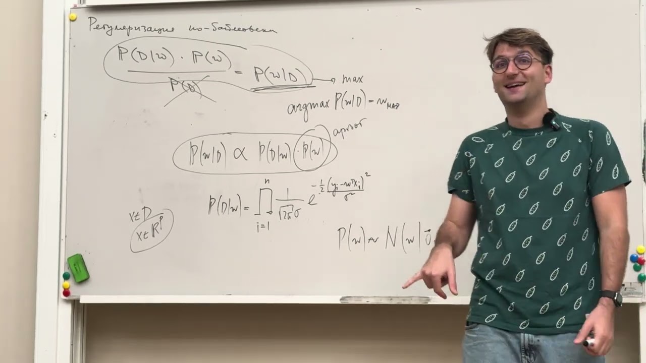
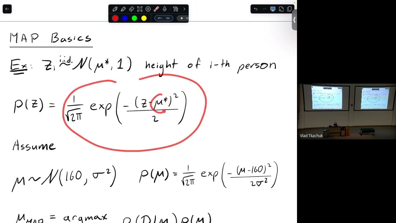
this question sorry it's still not clear to me why why why that is the correct goal to have to minimize the norm of theta how how is that so am i correct to say that we want to minimize the norm of theta because we want to not over reducing theta reduces yeah so the question is why why does reducing the norm of theta uh help um help or fight over fitting so the norm of the theta if you remember um this is equal to sum over i equals 1 to d theta i square right so the the idea that if you want to have small values of theta and you want you know all your values of theta to be small you know sum over the squared values and now that's that's the um that's the general idea right so you know if if all your thetas are are reasonably small then you get a a smoother function so you know penalize penalize those values right so um however this seems a little arbitrary uh i mean you know it seems a little hacky we just we knew we used our intuition to that large values of theta kind of cause over fitting so let's directly penalize it which which seems kind of a little hacky but however regularization has a very very nice bayesian interpretation right if you remember if you remember in the in the bayesian setting we had theta come from some prior distribution right and your data i'm just going to call it s for both x and y's so s given theta is something which is called the likelihood and we construct the posterior is called the posterior right in in the bayesian setting all we did was construct the posterior distribution so p of theta given s is equal to p of s even theta times p of theta over p of s right and this gives us a full distribution over theta and we use this distribution into test time to construct the posterior predictor distribution of you know for constructing p of y star given x star comma x y was equal to expectation of theta let's call it theta hat sampled from p of theta given s of p of y given y star given x star times p theta hat right so we constructed the posterior predictive distribution from from the posterior distribution however only in simple models is this integral tractable in most cases this inter this integral is not tractable it's very hard to perform this integration to construct a posterior predictive distribution let alone the posterior predict distribution it's very hard to construct even the posterior distribution of the parameters itself in simple models it's possible we saw that in bayesian linear regression it's possible but in a lot of other models constructing this posterior is extremely hard so what's done in practice is and this is something that you have on ps2 as well is something that's called map or maximum a posteriori parameter estimate right so what we instead do is take our posterior distribution right this is now a distribution over your parameters it is not a single point estimate it is a full distribution over all the infinitely many possible parameters and out of this we extract just one parameter setting called map which is the arcmax so theta hat map is the arc max of theta of from the posterior what is the arc max of so if you have a distribution over this theta this is p of theta given s what we want is to find a point which maximizes p of theta given s okay so we want this to be our theta hat map so the map estimate is the mode of the posterior distribution right the value of the parameter that has the highest density or the probability in the posterior distribution and and now once we once we obtain this we are going to switch back to the frequent test setting and make our prediction using h theta at m a p on unseen examples x star right so this is called map estimation and what we are going to see now is that regularization is essentially doing map estimation with particular choices for the prior distribution right well let us let see what what exactly we mean by that so what we were doing before was not taking the mean of this distribution we were holding on to the full distribution to construct the posterior predictive distribution right we were holding on to the full distribution to construct the the posterior predictive distribution right now we are not holding on to the full distribution we are going to just pick one value of theta and switch back to the frequency setting of using that as the estimated value this question it is very similar to mle and that's what we're going to see and that's what you're going to show in your homework as well it's it's it's so what we want to do is theta hat equals r max i'm actually probably doing some of your homework here for you so now pay attention p of theta given s right and this is equal to arg max of p of s given theta times p of theta over p of s right but p of s has no theta uh term in it so this is just arg max p of s given theta times p of theta and you can apply the log here because log is monotonically increasing and you get r max theta log p of s given theta plus log v of theta right so this is the map estimate and now what we are seeing here is that we are trying to find a value of theta that satisfies this times this right its trying to balance out two different competing weights if p of theta is gaussian normal with some covariance or sigma square then it is going to be your original likelihood term so this is your likelihood and this in case of p of theta to be gaussian as we have seen before will turn out to be some constant times lambda square remember the log likelihood of a gaussian exp minus half if it's mean 0 then it's just the square over here and you take the log of this it's going to cancel out everything except the square and that's exactly what you see here right so having a gaussian prior on your parameters and performing m ap estimation is effectively the same as adding a reg a squared an l2 regularization on your on your on your mle estimate so this could be in case of regression this is the square loss right and there is also ah you can you know do a quick visualization of this so if this is your theta and this is 0 then your prior is some distribution that's so this is prior and over here let us say this is your let let's call this likelihood right and this is your mle estimate so mle maximizes the likelihood right so assume this just peaked over here and instead what you're trying to maximize is the product of these two right the the prior times the likelihood and how how does the product of two functions look right so if either one of them is very close to zero then the product is zero right so over here the prior is close to zero so the product will be zero over here the likelihood is zero so the product is zero so instead what we get is so this is prior times likelihood right is the prior times likelihood because in any place where either of the prior or the likelihood is zero the product will be very close to zero so only in in the region where both of them are kind of non-zero that's where the maximum will be observed and map estimation will get us this one here right so theta hat map right so what we see is that m ap so there is this kind of um there is this conflicting forces between the prior trying to pull the parameter estimate close to zero and mle trying to estimate you know pull it towards what the data tells us the the estimate is and map is kind of trying to you know find the right balance between the prior and the likelihood and it's going to therefore shrink your mle close to zero right yes question statistics when you invasion statistics when you choose a prior for your parameters you choose the family and the parameters so the the initial belief ah is basically captured in the parameters of your theta uh the theta prior so if you have a strong belief that your parameters are close to zero then you will assign a very small variance which means your prior is peaked and if your prior is peaked at zero then this pull is even stronger and your map will be even closer to zero and sometimes it's common to use something what's called as a flat prior which means your prior is just flat which means your likelihood multiplied by the prior is going to hold the same shape so that's when you use something that's called a flat prior where you don't want to do anything at all but in that case you know you don't have the regularization interpretation for the regularization interpretation your prior needs to be a gaussian and this lambda is is going to you know involve terms of the you know sigma square and and few other things which you do in your homework but the general idea is this you know um you know this this acts as a regularization term because of the squared error that comes out here yeah so how confident we are depends on what kind of uh variance we assign to the prior all right um uh if there are any other questions feel free to walk up to walk up here and i can answer that and that's all for today thanks
Up Next

5:36
Coqui TTS Setup: Local Voice Cloning with Web UI
@Dev-Spot
19.2K views•2023-12-26

57:48
Secure Multiparty Computation (MPC): Foundations & Challenges
@SimonsInstitute
7.3K views•2015-05-28

104:31
Stanford CS229: Building Large Language Models (LLMs) | ML Lecture
@stanfordonline
1.8M views•2024-08-27

18:41
Neural Networks Explained: Math, Layers, and Learning Fundamentals
@3blue1brown
21.9M views•2017-10-05
Related Study Plans & Knowledge Roadmaps
Structured learning paths in Artificial Intelligence
artificial-intelligence
Aligning LLMs: DPO, TRL & Custom Datasets
01Foundations of Python & Machine Learning
02Transformers and Large Language Models (LLMs)
03Aligning LLMs: SFT and RLHF
+ 3 more learning modules
24h6 modules
Explore Roadmap
artificial-intelligence
Federated Learning: PyTorch, Flower & Privacy
01Python & Machine Learning Foundations
02Deep Learning Basics with PyTorch
03Introduction to Federated Learning
+ 2 more learning modules
35h5 modules
Explore Roadmap
artificial-intelligence
Securing LLMs: Guardrails AI & NeMo Gateway
01Introduction to LLMs, Python, and APIs
02Understanding LLM Vulnerabilities & Threats
03Defending LLMs with Guardrails AI
+ 2 more learning modules
15h5 modules
Explore Roadmap
artificial-intelligence
Building Recommenders: Two-Tower & Vector DBs
01Foundations of Python & Machine Learning Basics
02Introduction to Recommender Systems
03Deep Learning & Representation Learning
+ 3 more learning modules
75h6 modules
Explore Roadmap