

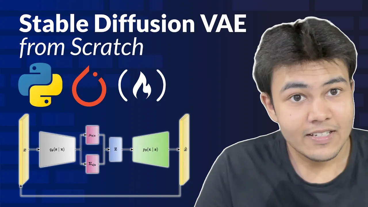




















Stable Diffusion achieves efficient high-quality image generation by performing diffusion processes in the latent space of a pre-trained autoencoder rather than directly in image space, which dramatically reduces computational requirements while maintaining image quality; the model architecture consists of an autoencoder trained with perceptual loss and adversarial training, followed by a UNet-based diffusion model that predicts noise in the latent space using cross-attention for conditioning, with sampling accelerated through the PLMS (Pseudo Linear Multi-Step) scheduler that connects diffusion to differential equation solving.
Stable Diffusion Code Explained: High-Resolution Image Synthesis with Latent Diffusion Models | ML Coding Tutorial
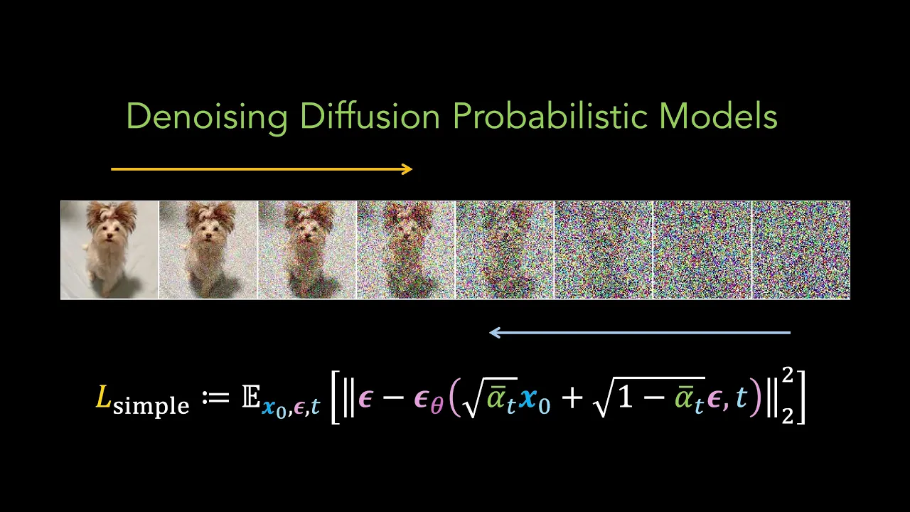
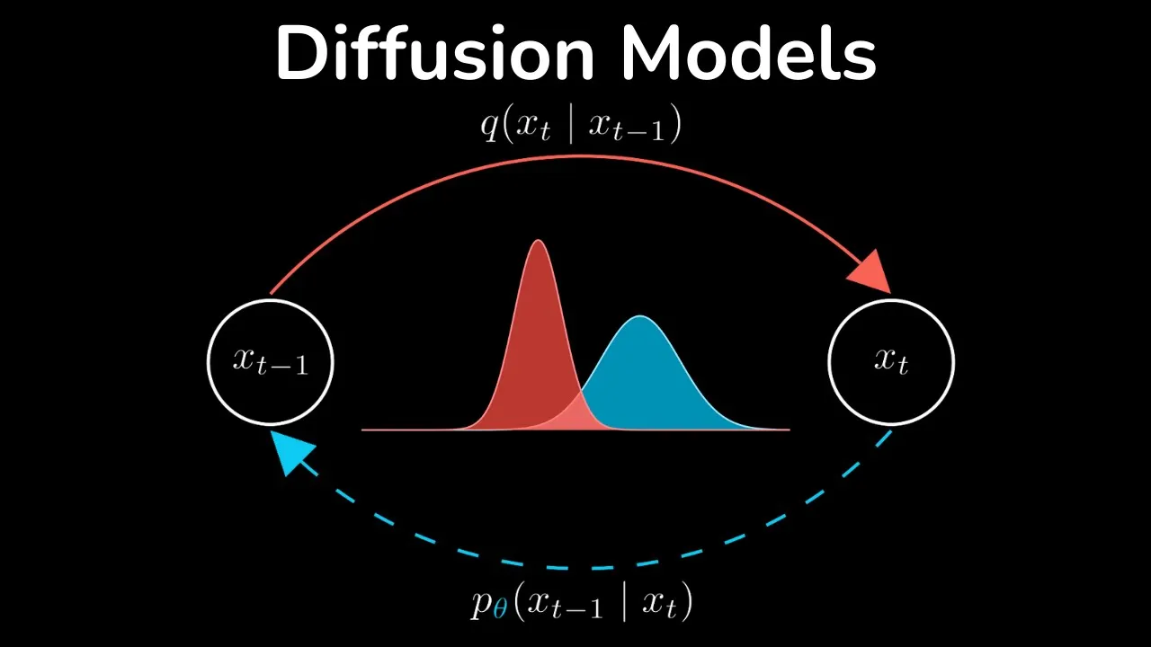
Added:Fundamentals of Diffusion Models (DDPM): Understanding the mathematical principles of the forward noise process and the reverse denoising process.
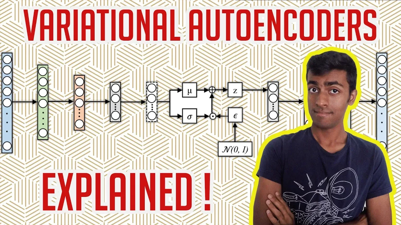
Variational Autoencoders (VAEs): The concepts behind compressing high-dimensional image data into a compact latent space and reconstructing it back to pixel space.
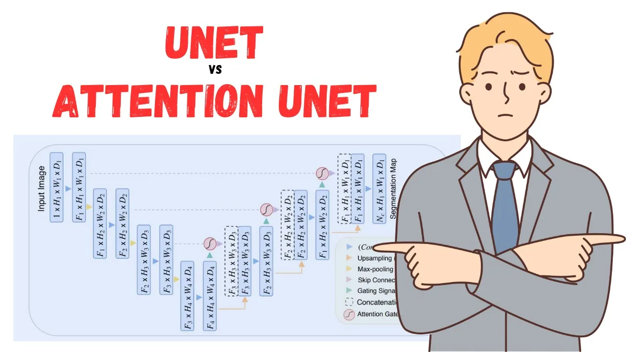
The U-Net Architecture and Cross-Attention: How spatial features are processed in deep learning and how external conditioning (like text) is integrated via attention mechanisms.
PyTorch Framework Proficiency: Practical experience with writing custom training loops, managing neural network layers, and manipulating multi-dimensional tensors.
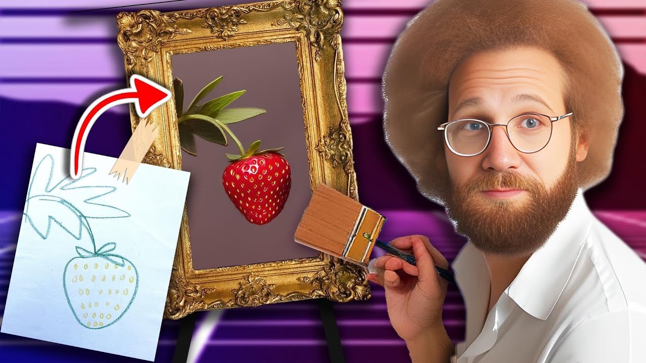
Parameter-Efficient Fine-Tuning (PEFT): Implementing techniques like LoRA, DreamBooth, and Textual Inversion to customize diffusion models with limited training data.
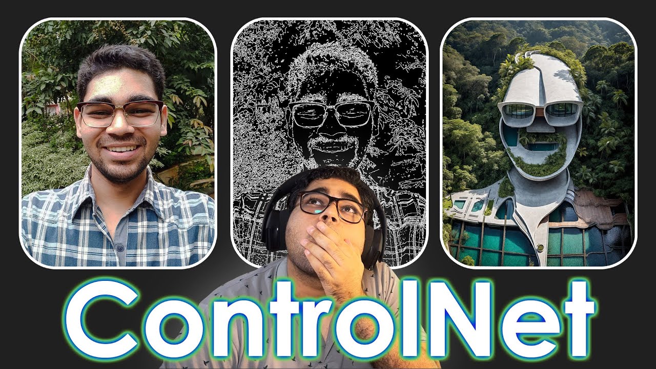
Controllable Image Synthesis (ControlNet): Studying how to integrate secondary neural networks to guide image generation using structural inputs like depth maps or human poses.
Advanced Samplers and Distillation: Exploring faster ODE/SDE-based solvers (such as DPM-Solver) and step-distillation methods (like Latent Consistency Models) to reduce inference time.
Multimodal Scaling (Video and 3D): Extending latent diffusion concepts to temporal dynamics (text-to-video) and spatial synthesis (text-to-3D asset generation).
57.4K views1.3Klikes1:40:35Original Release: 2022-09-01
what's up guys Alexa here in this video we are doing a deep dive into stable diffusion model and by the end of this video you'll understand exactly how the training of both stages Works how the sampling Works how to generate images etc etc having said that uh a week ago the wait for the stable diffusion models were published which is super exciting so we know that since the beginning of this year with the release of the W2 paper we had a Cambrian explosion of various uh image generation models such as uh well Dolly 2 we had mid-journey we had imagine party we had Dali mini which is the open source implementation of Adali version one uh etc etc and the reason why this model is so important is well there are multiple reasons one of them is the images are super high quality and additionally if you have much less constraints so that means you can generate images of human faces you can also because the code is open source remove the safety features and generate whatever you want although I do not I I don't encourage you definitely to share malicious images across internet but if you want to experiment you can do that as well so that's kind of cool additionally and very importantly you can run this model directly on your machine even if you only have a like a GPU that has eight gigabytes of vram so I personally have RTX 2080 on my laptop and I'm able to run this in flow 16 without a problem and generate awesome images in a couple of seconds so that's again very cool so it's much faster it requires much less memory and it has less constraints and it's high quality that's why stable diffusion is so so interesting okay so I want to showcase a couple of very cool examples that some digital artists such as Alexander here have been creating you can see how cool these uh these videos are and they were created using stabled Fusion you can see that the name of this piece is called Voyage Through Time and what Xander did and you can kind of go through the video and I strongly encourage you to check out this video it's amazing it's really like mind-blowing uh like that we can create this on like literally consumer grade gpus and and yeah and enjoy the this piece of work piece of art okay so here is uh an example of um the the prompts and the seeds Alexander had to create to generate this this cool video so you can see there is a lot of like CDs being used as a hyper parameter you have to tweak the seeds you have to tweak the the problems do some prompt engineering and at the end you end up with something as cool as as this video okay so I said I also managed to to run this uh stable diffusion on my GPU that has eight gigabytes of vram I was generating using uh float 16 Precision but you can see the images are super high quality as well so uh yeah these these images were generated using a prompt a pinning of an AI robot having an epiphany moment uh and additionally I'll I'll basically um release a script that I use to generate uh some cool um like some cool interpolation so basically the idea is to you you pick you generate the diverse set of images such as the set you've seen here and you can pick two images you like and then basically do interpolation between them in the latent space uh of the model so that was inspired by about these uh just but yeah I'm gonna share that that script very soon and also cover it in a different video so you can see here how it looks like the interpolation between basically I'm interpolating between this image here and this image here and I'm going to now show you how how that procedure kind of looks like so here is how the image is being morphed as we're approaching the target image and you can see there are some like uh jumps uh in the latent space but all in all let me kind of uh move this faster you can see how how cool it is uh and yeah I'm gonna share this script a bit later so having said that uh let's jump into the um uh the code and well first let's let me show you some some prerequisite knowledge here uh I'll have three papers which I'll consult I will not do deep Dives of the papers in this video so one of those papers is um a theming Transformers uh basically for high resolution image synthesis that introduce the VQ gang paper uh I've previously covered that paper on my on my YouTube channel so do check it out if you want to have a thorough thorough understanding of how that works I'm going to consult some of the formulas later when I show you the code uh next up we have the high resolution image synthesis with latent diffusion models or ldms and that's the paper that's behind the stable diffusion model basically so ldms is what's powering the stable diffusion and finally I'm gonna briefly um consult this paper pseudon numerical methods for diffusion models and manifolds that introduce the plms so the pseudo linear multi-step scheduler that makes uh stable diffusion fast and high quality so you can literally have only 50 steps uh of the fusion model and still generate very high quality images okay so I'm going to briefly walk you through through some ideas in this paper like super briefly and if you want to learn more about the fusion models they have a whole like a diffusion playlist so do check it out I've been doing both the paper overviews as well as as code walkthroughs of the original repos so do check those out if you want to have a deeper understanding of how the fusion models work here I'm gonna do a mostly a diff between what has changed compared to those older models okay let's start here so to enable to enable diffusion model training unlimited computational resources while retaining their quality and flexibility we apply them in the latent space of powerful pre-trained audio encoders so this is literally the main diff compared to all of the other papers they train instead of of working in the image space and doing the forward diffusion process and then low learning the reverse process in the image space instead they do that in the latent space okay let me just quickly show you the difference in the loss so here it is so here is the original uh basically construction how the original loss for the ddpm model looked like you basically do you sample images here you sample uh noise from the from the normal distribution you sample different time steps and you literally just do MSC loss so the mean squared error loss at between uh the the noise and what you predict so this is so Epsilon Theta is modeled usually as a unit architecture so using the unit architecture and so what you do is take the x of T which is the original input image plus T steps of diffusion being applied to it so you kind of noise it and then you pass this noisy version and the time step uh that's that so basically the time step information and then you need to to predict the the noise that was literally used to noise that image in the forward process if that makes sense so this is just a whole player recap for for most of you and then you just keep on repeating this until you train this unit to predict the noise and then later you can just use it to denoise the uh well uh Pure Noise images such that you can generate cool images okay so this is the only difference between ldms so that this paper and the previous work they are literally just working in the um latent space of this encoder uh and uh you can see everything else Remains the Same so literally the the difference is the following so instead of working in the image space you're going to um whoops you're going to have a like an encoder that's going to train been is going to be trained using the similar to Wiki gun paper you end up so you input the image you you end up with a latent here and then everything else Remains the Same You're Now using this latent to to train your diffusion models so here is the uh like a snippet from the ddpm paper uh so now instead of using X of T it will not be an image here it will uh it will be instead sorry X of zero will not be an image is going to be instead like a latent representation of the image and that's pretty much it really really that's all there is to it that's the only diff between this paper and uh and the previous art so here is how the how the diagram looks like so we will the Code walkthrough will contain at the three three parts the first part I'm going to show you how to train the auto encoder here it's going to be the first part of the video the second part I'm going to show you how to train the unit so the fusion model such that uh you can so you can see here we we first end up in the latent space then we do the forward diffusion process such that we end up with Z of T and then we diffuse it we will learn how to predict the noise that was added during this diffusion process here we'll learn how to predict it as the output and uh well that's it everything else is the Future Magic and also we'll have I'm going to show you how how they are using it the we'll also be learning the conditioning model so we'll mostly be focusing on text as well as classes from the imagenet data set okay that's it and the third part of the video will be about basically how to sample once we train these models if you didn't understand everything uh because you lack some background uh feel free to continue watching this video I think that the code will be fairly self-explanatory um Okay so if you want to follow along uh what I'm doing here you'll have to do a couple of steps obviously you have to clone the original repo so the stable diffusion repo here just create the current environment following the instructions here under the requirements section and after that go ahead and download uh like such that we can have a minimal setup and just get something running uh you don't have to to download the original imagenet data set which is huge you can instead go to this uh like Fast ai's image net however you pronounce this thing uh like uh GitHub repo and download the smallest version possible so literally it can't be 60 pixels it's gonna download only 10 classes from imagenet and it's going to make us uh well uh set up for for for for the training procedure um basically this older repo latent diffusion which preceded their stable diffusion repo which I'm going to also Link in the description contains the necessary instructions for how you can unpack uh the data set and where you need to place it such that the script can can recognize and the data can be loaded uh okay guys so let me jump now into the actual code here we are a couple more things we need to sort out so first of all obviously we need to set some input arguments there is only a couple of them that we care about first one is we want to pass the uh like the the the the the the configuration file for the auto encoder so first we're gonna train the odd encoder and then you need to pass the T flag meaning we want to train it and then gpus so I'm passing zero a comma because I only have a single GPU and the index of that gpu0 if you have multiple gpus feel free to add one two three whatever how many gpus you have there okay final thing because this is a research code base after all uh there are some bugs and so I had to kind of sort them out before getting this to work on a Windows machine okay so let me open up my my diff tool here so I just have to do this get div tool B and I'm going to open up uh the differences to the code I made so first of all um this is not a bug uh this is just like a small modifications you have to do if you want to train this on a single GPU if you want to be able to do a walk through on a vram limited system so basically uh set batch size to one instead of default 12 otherwise you'll get Cuda out of memory exceptions that's the first week you have to do the second one is actually a bug so you have to go to data imagenet file uh I mean it's a bug if you're on windows so the thing is they kind of hard coded the slash here assuming that that's how you split the path on arbitrary system which is not the case for Windows so it's much better to use os.sap which is going to resolve automatically depending on the operating system into the correct character sequence for Windows that's going to be double backslash and so this now works otherwise you'll have some errors and the the training will not work okay and the final tweak is in the main script so if we go here to the main script you can see I had to make a couple of changes first of all I had to set the number of workers to zero because otherwise I was again getting some some errors um that's one tweak the second week is set the shuffle to false here uh for the train data loader the reason being is uh we are using if you recall we're using that super small uh sub sample of the imagenet and so if you just keep if you just do the shuffling it might happen that you take some super big index and try to index into our data set and we don't have that image and then you're gonna get you have the uh well index out of range exception or something okay so that's the second week I had to do um the third week is comment down the DDP in case you only have a single GPU so that's the distributed data parallel uh like a object from from pytorch I don't need that so I had to comment it out and finally I had to comment out the signal Parts because that does not work on Windows and I didn't want to bother figuring out how to fix it on Windows because I'm just gonna I just want to do a walk through and explain you guys how this training procedure looks like that's it we are ready let's get into the code I'm gonna start in the main file so main file is the is where the training magic happens so let me go to the main function here okay so here we are I'm gonna set the breakpoint here and uh let's start debugging this thing okay so just hit the training we're going to use the information we passed in our launch Json if you're using vs code if not you just need to pass those arguments Somehow Here we are and again I'm going to focus only only on on important parts so I'm going to skim everything else like we're just doing some parsing uh blah blah blah we can skip literally everything we're just creating some directories doing some configurations I'm going to skip here this is a Salient point so here we are doing the like loading from the config file so let me show you briefly how the config file looks like so if you go here if you find the configs directory and then you find under the auto encoder you'll find the one we're using so that's this one and you can see everything you need to instantiate various sub modules of the of the ldm is here so we have the auto encoder here we have the loss we are using we'll see what this is it's basically a perceptual loss and the parameters we use to construct it loss we have uh information to specify such that we can uh construct our data loaders uh some callbacks for pytorch lightning which is the framework they are using which is built on top of pytorch if you've never heard of it and that's it like some information about um accumulating radiant uh nothing nothing important let's go back to the um basically main function that's all uh you need to see okay now I'm Gonna Keep skipping all of this accelerators gpus nothing fancy I'm gonna skip all the way here to a model so that's where we instantiate the actual model okay so you can see here we're gonna now construct the auto encoder KL so uh let me just see whether I've enabled all of the breakpoints and if so let me do F10 and I'm gonna hit the init function of the auto encoder okay a couple of steps here we because it's an old encoder obviously we have to instantiate first the encoder and then decoder so let's see how those look like basically let me just see what this DD config is but I'm fairly yeah okay so it just contains the the necessary parameters to constructing color Okay so let's let's go into the encoder uh encoder nothing nothing really fundamental um basically a bunch of com layers a bunch of um there are some interesting attention layers which what basically what I do is in the latent space of the encoder so they take the image features and they just do the vat type of uh like a self attention so you kind of you can kind of unroll them and then just do simple um like a self-attention logic where every token attends to every other token that's it and then there's some down sampling layers uh which are again just a combination like basically you can see here just to come like a layer with a stride of two what not that's it uh I'm gonna jump over all of these again just a simple uh encoder model nothing nothing fancy there okay let's continue let's exit this part and now let's enter the decoder similar story uh nothing fundamental to understand here A bunch of com layers bunch of res blocks and then there's some up sampling I'm going to hit F5 let's exit this model that's it the architecture is not the interesting part of this of training the audio encoder um okay now this is the interesting part here's where we instantiate this lpips with discriminator loss it's a mouthful it's basically a perceptual loss combined with adversarial loss so let's step into it okay so here it is here we construct it again I'm going to focus only on the important parts we have some loss coefficients so depending on which component of the loss we are looking at we'll have a different weight but most of all let me let me show you this so if you're not familiar with this perceptual loss concept I think it has been introduced at least since the neural style transfer paper so that was the those are the were the first papers I saw were using the perceptual asset so the idea is to basically let me step into it to basically uh take a pre-trained vgg 16 Network and uh then pass your image and grab some in representation intermediate representation from the vdg16 network and then basically do MSC in the latent space in that representation space instead of in the image space and by doing that you can kind of compare like the semantics of your input images and not not like focus on on some maybe superficial noisy details in the image space that's the basic idea additionally there are these net lean layers which what they do is they reduce the number of channels from let's say 64 to 1 and then you can kind of collapse them and do the loss logic we'll see in a couple of minutes what that exactly means once we start doing the actual forward prop through the models now we're just instantiating so this is enough for you to understand so we are loading the model here and then we literally grab the pre-trained model uh from the uh theming so this is their older repo so taming Transformers that which introduced the vqam paper and they basically have a checkpoint there of the of the that that's going to initialize this LP IPS uh loss okay so let me just kind of go and do that and you can see here loaded pre-trained loss from this file here vgg pth okay so now what happens is we just set gradients to false everywhere and uh that's pretty much it so let me now hit F5 and we are out of that function okay now the second interesting part is discriminator so that's going to be used in the uh adversarial uh loss component of the final loss again um I'm not sure it's worth even digging through it but it's literally just a bunch of uh you can see here so there is some batch Norm going on come layers leaky real use come come layers leaky values nothing fundamental there I'm just going to skip over it and it's again going to down sample because this is a patch based um discriminator you can kind of check you can see here that's the patch can discriminator there was a first described in the Pix to pix paper uh you can check out this link if you want to check it out but the main difference is instead of having a scalar and then say scalar telling you whether this image is real or or fake which again networks too again discriminators do here you'll instead have literally for a patch you have maybe 32 by 32 uh scalars and all of those will will tell you so a particular uh scalar will tell you whether that patch is real or fake and that just kind of gives you more information to train uh so more information for for for your model to train that's it okay let's exit the discriminator again we have some hinge loss we'll see how that comes into into play a bit later we have this uh weights again okay we'll see all of that a bit later that's it now we Define some more calm layers uh blah blah blah nothing fancy monitor just tells us which loss are we monitoring and in this case validation reconstruction loss is something we care about okay that's it now I'm gonna skip again with some biases uh logging uh blah blah blah there is some model checkpointing we don't care about model trick pointing in this logic there is as you can see it's kind of Fairly uh well researchy code base some callbacks logging images learning rates blah blah Cuda callbacks nothing nothing fundamental for our understanding of how the how the stable diffusion is trained so I'm going to skip all of that until until I guess until the data part okay so it's gonna skip until the data part so this is where we load the imagenet data and again uh if you've set if you downloaded the uh the the image net n e t t e data set uh and you've placed it into the correct directory then everything is going to work as expected here plus the minor tweak I made with the OS separator if you recall that from a couple of minutes ago okay so again I'm gonna ignore uh all of this because it's just gonna prepare the data nothing nothing um fancy there so I'm gonna do this and click F5 and wait for our data to be loaded you can see there is some filtering going on blah blah and we have the data ready okay so that's it we have you can see here train data and validation data you can see the numbers are super super big and that's definitely not the number of images we have in our small imagenet and that's the reason why I have to set the shuffle to false otherwise you'll you'll get the index out of range exception uh again this is just what it's needed what is needed to get a minimal setup up and running if you actually want to train this then obviously you want to have a full image now you want to have multiple gpus et cetera et cetera but if you just want to step through and understand what's going on this is more than enough okay again I'm going to skip across all of these parts not too interesting checkpointing blah blah debugging signals I'm gonna uh enable breakpoint here hit F5 and this is where the magic will start going on so I'm gonna now enable all the breakpoints and let's start digging into this code okay so F10 we end up in this on pre-trained routine start so that's again uh something that Pi torch lightning uh defines for you um pytorch lighting is very cool if you're a researcher and you're doing something that's fairly has a fairly common structure in the sense that you don't have to think about zeroing your gradients you don't have to think about calling the optimizer step you don't have to think about all of those details you just have to define a couple functions that the um python lightning API uh requires you to and then everything kind of works out of the box uh automatically okay this part is not uh interesting we're just creating some directories for configs and logging nothing nothing interesting really and finally we hit the validation data loader now you may be confused why are we starting with validation how does that make sense and that's again pytorch lightning uh detail um what the framework does and I think this is fairly brilliant is it first literally loads only one or two batches of data uh in the validation Loop just to make sure that the validation works so that you don't have to waste bunch of time in the training Loop only to find out that your validation Loop is broken and then you have to start from scratch so instead of what they do is literally just verify that validation works and after that you resume the actual training and then validation everything else remains according to the usual um sequence okay so because of that I'm going to disable all of the breakpoints here just enable the one in the train loader hit F5 and wait until this validation data set uh basically check is is completed here it is um we can see we are hitting the train data loader again that's something that pytorch lightning requires you to Define let's continue here and uh let me just see whether I've enabled all the breakpoints okay so now we're going to first okay again some some some fighter lighting stuff okay so here we are so what now what's happening is we are loading the data from our training data set and here we are we end up with this example we've done some pre-processing you can see here we fetched the image blah blah blah and we end up with example which is a dictionary that has multiple keys so image and other imagenet um idiosyncratic uh like uh keys so let me show you some of those so example image is obviously our input image so it's process such that we have 256 to 56 and three channels we also have if I do example let's say class label whoops I need to make it a string so class label it's going to be as you can see label zero so our data set only has 10 labels we are not using the full image now that's why zero is highly probable uh then let me show you one more human label obviously just a human readable label of this uh imagenet class so Tinka Tinka whatever that is and that's it okay and this is where it starts getting interesting so so here we are we have a batch that was provided to us by by Patrick lightning again we have image in there the shape is familiar 256-56 and now we we do this uh get input it's just going to fetch the image do some permutation make sure that the memory is contiguous blah blah blah and now we're doing self and we pass inputs so this is a fancy way of saying call the forward method of this class and let's see so we are dealing with we're dealing with other encoders here obviously and uh the forward class is here so let me just do F10 and we hit this part so first part is obviously we do decoding and then we do the sampling and then we do the decoding okay um so let's dig into the decoder here it is here is the decoding logic some down sampling blah blah again I'm going to skip everything here because as I already told you encoder logic is fairly simple we just do a forward pass through it and we end up with a latent space representation okay so let's see what's the dimensionality of this uh representation you can see it's 6 64.64 and we expected three because if you recall let me let me show you the well we're using such a config where we expect 64 64.3 uh six is there because we are actually returning the mean and the standard uh the deviation or the variance uh here uh and uh then we're sampling before we passed that sample to the decoder so that's just a detail uh worth mentioning they did experiment with different types of Auto encoders one of them we are currently working with is the KL regularized odd encoder they were also playing with quantized versions but we really don't care about all of those details there is just too many things going on okay some processing of that representation we end up with moments when when they say moment they literally mean zeroth and first moment like so the mean and the and the and the variance so now we pass that into this diagonal gaussian distribution so we're gonna basically form a distribution here we're going to name it posterior so let me kind of enter there you can see we just uh Chunk we just split into two parts uh that representation and we end up with mean and log variance so that's what we're actually returning and then some clamping exponentiation such that we end up with standard deviation variance and that's it okay just a gaussian that's all after that we have the sample and sampling is simply because gaussians are such a such a nice mathematical object you basically just have to take the mean and add to it standard deviation multiply by the normal noise from the normal gaussian that's it okay and we end up with the representation so now let's see that should now have three channels I guess so 364 64 as expected okay so now let's pass this into the decoder stage here we are we do some processing just a com layer uh decoder what it does is again just up sampling conf attention again trivial stuff I'm gonna skip over that that's kind of um common knowledge okay so we end up with output output should be because this is an auto encoder should have the same shape as the input image so that's 256 256 3 Let's just print out the shape so that we are yeah okay we can we can see here that the shape is as expected let's continue we now return that decoded output and we return the posterior object which is the gaussian and that's this part okay so now you'll see there are two if statements here one is when the optimizer index is zero and the other one is when the optimizer index is one the reason we have uh those parameters is because we have two different optimizers let me just see whether where is that function so configure optimizers I I didn't show you this one so we didn't step into it but simply uh simply put we have two optimizers one is atom and that atom is going to be optimizing encoders and decoders here and the second Optimizer is going to be optimizing the discriminator weights so we saw that when we instantiated that the discriminator I told you that it's going to be trainable and here the other Optimizer cares about updating discriminator weights whereas this can be treated as a generator so the auto encoder part is the generator the discriminator is obviously the discriminator and that's that's it okay so let's go back here so pytorch lightning makes it easy for us to do this type of uh again um loss computation so first we'll step into this branch and then it will literally return called the training step again with Optimizer index set to one and then we'll train the discriminator so that's everything is kind of handled for us by the framework okay this is where the whole brain of this Auto encoder training is going to happen so let's dig into this code this is very important uh okay so we get the last layer that's going to be used for some Lambda calculation you'll see that in a second so here we are we are inside of the loss let's see how the loss looks like for the other encoder so first of all we have the Reconstruction loss it's simply as you can see here we subtract the inputs which are the inputs image so let me let me just kind of make sure that this is numpy or Pi torque tensor I guess yeah and then let's just see the shape the shape should be at 256 yeah everything's fine there we have reconstructions we literally just subtract them and we obviously want to make this difference as small as possible so that makes a lot of sense we're just doing Simple image space um like MSC type of a loss okay now we have perceptual loss this is the interesting part so we pass the inputs and the reconstructions again but this time we do not compare them in the image space instead We compare them in the latent space of the vgg of the pre-trained VG Network so let me show you that thing as well okay so here we are so we are again in this LP IPS uh loss and we are in the forward step so first thing they do is they have the scaling layer and that scaling is just going to subtract some mean and so let me just find that for a second so scaling layer is here so literally there's some shift and scale um so uh computations going on I'm not sure whether this is from imagenet statistics or not like if somebody knows let me know I think this is from imagenet and that will make sense since we are now using imagenet data set as well so that would make sense we're just going to normalize our input tensors and then we pass them through the vgg and so you can see here what the vtg4 passing in uh entails so literally we're gonna return some intermediate representations and we're gonna wrap those up into this named Tuple object and return it back so let me hit F10 we are here we're going to return all of that we're gonna hit it again because we have two computations both for the input as well as well as for the Reconstruction now we kind of uh cluster all of these layers that are going to reduce the number of channels together just some syntactic sugar and finally let's see here is where the magic is happening so what we do is we normalize the tensor normally it's just gonna basically divide it by the L2 Norm okay and then we do as you can see here again we just do uh we do we we subtract them and we do the square so it's a MSC loss without the M part because we're not doing the mean part yet we're just doing this and we repeat that for all of the representations because we will have like five representations from the vgg so that's why we'll have five iterations of this Loop and now we're gonna break out of it and now we're here okay so now what happens is we are going to pass those differences into these layers that are going to reduce number of channels so let me let me let me let me explain what I mean by that so here here is this stiff so here is the difference in the that we that we've done among the features and the shape is going to be what so here's the shape after we apply this layer so after we apply this we'll just end up with a single channel so if I put 0 here and if I put 0 here and if I just do the shape you can see we have 1 1 256 256 okay so that's the sole purpose of this of this layer and finally we do the special spatial average which is simply a mean amine across dimensions and so we end up with a scalar here and that's it that's that's how the perceptual loss looks like it's fairly simple uh and I'm gonna just keep on stepping over five times there and then I'm going to hit F5 and that's it so now we end up with uh this this array of um well it's actually yeah we've accumulated we've up aggregated the values here by doing the sum operator and we end up with a single number and that's the perceptual loss that's it guys um the only part that's kind of new here for me personally are these layers you could as well skip that part and simply do uh like a mean operation across these differences so just MSC loss uh directly in the feature space and that's it but this is some type of a modification I'm not sure why and where there are some ablations but okay that's the perceptual loss okay finally we've formed the the Reconstruction loss as a weighted sum of the Reconstruction loss from the image space plus we we grab the perceptual loss here and we have some weights 1.0 here okay so they are equally weighted okay next up since this is zero this is going to be zero let me just kind of double check and because of that exponent raised to the power of zero is one so it's just gonna be a neutral operation so this is doing nothing and this is also going to skip here and here we just do some uh rescaling that's it summation blah blah blah and that's our final reconstruction loss that's the the loss there uh now we do the because remember we return the posterior which is the uh gaussian from the latent space of the audio encoder and we're just gonna compute the KL Divergence so that's going to be the regularizer component so I'm going to hit F10 here you can see it's Simply Computing the KL Divergence using the mean information variance and log variance information okay and we end up with a KL loss there summary scaling again and now we enter the the branch where we train the generator I assume let's see okay all is good so far okay so we passed the reconstructions which are the fake images through the discriminator and we get logic it's fake okay and then what we do is we have a minus and we do a mean across those weights so let me show you the shape as this as I told you that's a special discriminator that's like a patch based discriminator so that means that the shape is going to be maybe I think it's 32 times 32 or something so let me see that so it's 30 30. so that's how many patches we have and we just do a mean across them and by putting my minus here we are literally forcing uh we will be tweaking the generator weights in such a way such that the discriminator gives a high value which means it thinks quote unquote that those images are real so again that's just your your Gan standard again stuff not nothing nothing super complex there if you're familiar with Gans uh okay and uh now there is some adaptive weight calculation let me see uh so what's going to happen there okay yeah so I remember this is going to uh make make sure that we we are waiting the the Again part of the loss and the Reconstruction loss appropriately let me show you uh the paper formula for this one is going to make a bit more sense okay guys here we are this is the vqam paper uh I showed that in the beginning of the video and this is basically the formula we're Computing uh we are taking the gradients of the Reconstruction loss with respect to the last layer of the decoder weights we divide that by the gradients of the gain loss with respect to the weights of the last layer of the decoder again what's the reasoning behind this the reasoning is the following if the gradients are super big for the Reconstruction loss and they are smaller for the gain loss then this is going to be a big number which is going to going to put a bigger weight on the gain loss so by doing that we make sure that the network is learning from both losses and that one loss is not overwhelming the other loss when it comes to the contribution to the gradients so that's the the rough logic and you can see um that that's exactly what we're Computing here so you can see NL loss so it's the Reconstruction loss of the last layer weights and that's it we get the gradients there then we compute the gradients for the gloss which is the Gan loss that's it and now we just normalize them we do the norm we divide them as well and that's it there's a clamping blah blah blah times some weight and that's it that's the that's it weight okay I'm now gonna return back to the code here now this is gonna be zero for the initial 50 000 iterations or something uh the reason being they don't want to they first want to train the auto encoder and ignore the the Gan loss such that they can form some representations and for the stability sake and only then slowly start using the Gan loss so let me let me show you what I mean by that let me enter here you can see that until we pass the global threshold so I'm gonna enter here you'll see that the weight will be zero so the weight will be set to zero until the global step uh crosses some certain threshold and because of that this is zero and you can see it's used here so that means this thing is kind of toggled off for the good portion of the of the of the of the beginning of the training so that means we only use the KL uh regular regularizer loss here and we use the Reconstruction loss here as the fine loss that's it I know this was a mouthful but like hopefully it makes sense uh now we just do some blah blah accumulation of those and we return back the loss and that's it we do some logging we return the auto encoder loss and that's it now we're going to hit the training step again this time we're going to be training not the generator but instead we are going to be training the discriminator let's see how that's gonna look like again uh blah blah blah I'm going to skip across these steps I'm gonna do uh basically wrong disable breakpoints we're gonna do a forward pass again uh this is kind of sub-optimal the there there must be some way to optimize this such that we don't have to do because we are basically sending the same images here again and that doesn't make much sense and now let me let me return let me enable back all the breakpoints now we enter this this Branch here okay so again we have a loss here all of the inputs are the same uh what's different is that um let me just enter here so we're gonna have the same Parts here reconstruction loss everything else Remains the Same so the interesting part that we care about is here so we want to go here so I'm gonna disable breakpoints enable just this one hit F5 and we enter this Branch this time okay so here we are now we pass the inputs to discriminator to get the real images and we pass the reconstructions to get the fake images the largest of the fake images okay again we just have this uh factor which is going to be zero initially which means this loss will not be uh enabled in the first part of the training and later it's gonna gradually kick in and uh basically what we do here is a hinge loss between the Logics of the real and the fake images and uh basically that's it that's that's the gain loss so this is going to train the discriminator such that the discriminator learns the difference between real and fake images consequently that's going to lead to better audio encoder because we're we're losing that we're using that discriminator to train the audio encoder guys that's it that was the training of the other decoder hopefully that was interesting and uh and made sense and now I'm gonna just stop this training because that's pretty much it okay I've hit F5 just to show you that now we're just gonna iterate across patches and keep on repeating the same things we've just seen so that's why I'm gonna stop this training right now uh we've seen how the auto encoder training looks like I'm gonna show you quickly the formulas from the vqam paper just to to consolidate the knowledge here and then we're gonna step into understanding how the diffusion the unit model is being trained okay guys quickly uh coming to the paper uh here are the formulas for the vqam paper so um originally how the VQ gun was trained was it had these code books of discrete uh basically vectors and they had the Reconstruction loss component you can see here plus uh these losses here uh were called commitment losses and they were used to train the code book uh and the encoder what changed in the week again is that they started using so you can see here um they're using instead of L2 loss they use a perceptual loss and they introduce an adversarial training procedure with the patch-based discriminator so that's everything we've seen so far and you can see that the final loss looks like this so there is the the again component weighted by this Lambda we've seen all of these and then there is this component here that basically consists out of the Reconstruction loss and the perceptual loss and additionally in this uh in the latent diffusion model they've introduced the KL Divergence regularization so basically bottom line is the order encoder used for the ldm paper is a small modification of what they've already done the same authors in the vqam paper that's it let's go back to the code pondering uh for a second about why these losses make sense even though they are but they are not by any stretch of imagination probably an optimal solution to how we should be training our models but let's just think about it for a second so we have the Reconstruction loss in the image space and we have the perceptual loss those basically make sure that we are we are reconstructing images correctly so that we can we'll learn how to uh not lose information when we go through the bottleneck part okay then we have the the again component which makes sure that the images look very realistic so that's additionally kind of enforcing uh the reconstruction and finally we have the KL uh Divergence loss that's just going to be regularizing the the the latent space of our old encoder such that we can later be able to smoothly uh go through that space and be able to uh have meaningful uh representations so that's the basic idea like we are yeah okay having said that let's go to the launch Json let's modify the the the the argument such that we are now training uh we are now training the um diffusion part and not the audio cutter so I'm just gonna remove this part here uh remove this space here and paste this back here so that's everything you need to do now we're training the um diffusion model so let's go back here the difference will now be that they are not using with this config they're not using the same mod encoder they're using a different one with the with the quantization but like that doesn't matter we're going to focus on on important parts only okay so I'm gonna um hit F hit the training here and let's start analyzing the code again I'm gonna Focus only on on instantiating the models and on the training Loop that's it I'm going to skip everything else because we've seen all of that we've seen the the config as well so let's just go to the model instantiation so let's go here and now let's uh let me just make sure that everything is enabled I think it already is but yeah okay so here we are latent diffusion uh like object we're starting to instantiate uh everything we need so one of those things is going to be a unit uh architecture okay so let's start here let's see what's going on we can ignore all of this so here is the first interesting part we're going to be initializing the superclass and the superclass is this ddpm okay so the ddpm is the uh denoising diffusion probabilistic model so that's the original diffusion paper that made diffusion kind of practical okay so let's enter there so let's see what's going on there okay so here um we are predicting you can see we're running in apps prediction mode which means we're predicting that uh noise uh instead of uh well there's some other things you can predict like x0 uh Etc okay we can skip all of this we can skip all of this now there is this diffusion wrapper um and that that's where we actually start making the unit so here you can see here unit model is constructed here so let's construct the unit let's see how it looks like again in some of my previous videos I've been going through in a lot of detail through how unet is constructed so you can go through that if you want here I'm just going to kind of quick a scheme and by the way I love the I love the statements in this in this uh code base full you forgot to include the dimension of your cross attention conditioning very cool yeah you can you can tell it's a production code okay so let's let's continue here I think we can skip across all of these details um the important parts are these time step embed sequential objects what they basically make sure is that uh we can later pass uh time step information or or a conditional information into various sub modules so let me kind of Click F12 there enter the definition you can see that depending on the layer uh type they'll sometimes be passing the conditioning information sometimes the embedded information sometimes just the input features image features and that's it so it might be interesting to for me to just show you one small thing and that's the following so there are these blocks that integrate the conditional information and I think those might be interesting so here spatial Transformer so that's the module that's going to be integrating the conditional information into the unit so I'm going to hit F12 there and I'm just going to add I'm just going to add like uh basically a breakpoint there and let's hit F10 let's continue everything else we don't care about really we can just construct the unit and let's go to the end here so this is the end of the unit definition quite a long definition definition as you can tell so I'm going to skip over it and that's it so we're using cross attention to do the conditioning the conditioning the conditional information integration uh so yeah okay okay so let's continue here okay that's it uh counting the parameters nothing fancy we don't care about that as well that's just the exponential moving average um not not the fundamental part why this model is working so I'm going to skip across all of these uh now we're registering the schedule so this is the important part and I've covered uh how this exactly works like for I've been doing side by side comparison of formulas and uh of of code so do check out I'm going to link those video cards somewhere here but the diffusion playlist is the best place to start if you want to understand a bit better why those work otherwise this video will be like five hours long or something so let me let me enter here uh let me just show you how this roughly looks like so you can see here A bunch of those Alphas uh and uh Alpha like the cumulative products and and uh all of those variations of the formulas basically nothing is learnable here uh these are just the weights of the scheduler that we need to get the fusion to Brick so I'm gonna skip across all of these and that's it that's an important part but like something I've covered previously and uh just a bunch of formulas you wouldn't get any insight from me going through it so yeah uh I'm gonna skip over that okay we are back in the latent diffusion so we we generated the uh unit we generated a schedule now let's continue and see what else is interesting here I'm going to skip across all of these so because now we are training the the model in a holistic fashion we obviously have to instantiate the first stage and by first stage they mean the auto encoder so let's again just briefly go through this one this time we are forming this VQ model and not the auto encoder KL so that's a that's a difference so let's just do that so here we are uh we are instantiating the the the VQ model here we are and that's gonna call the VQ model here so let's just kind of start entering there okay so here we are um let's see what's the mean difference we still have the encoder I'm gonna just toggle off all of the breakpoints uh we have the encoder we have the decoder nothing can change there the only difference is so we have a loss which is going to be identity in this this time because we are not training the odd encoder we'll just be we'll be just loading the pre-trained weight so let me enable all of the breakpoints and let's uh enter this part so let's see what's going on there some embeddings blah blah blah um well it's not blah blah blah embeddings are actually what's important in this model so this is a code book you can see there is 16 384 uh code book vectors and each of those has four uh dimensionality of four and that's what's being used to do the quantizations later in the forward step we'll see how it looks like a bit later okay so that's the Qantas part now we have the com layer same as with the auto encoder KL nothing has changed there uh blah blah blah we can skip that we can skip all of this and now we initialize from the pre-trained checkpoint uh I'm just gonna skim over all of that we are just basically doing the initialization of the order encoder because remember how how the whole logic works you first pre-train the audio encoder and then you basically freeze it and you use its latent space and now you train the unit and the conditional model and everything that's that's the idea that's why we're loading the the weights here uh okay and that's it now we do some uh set the eval mode and basically now we set the gradients to false everywhere and we can just continue on with the execution here let me hit F5 we exit the condition instantiate the first stage a function and now we instantiate the conditional stage so this time uh let's enter this one I think we are just going to have a class information so you can see here uh class in better is the type of a conditioning model that will be instantiating here so let's enter there you can see it's simply thousand classes because we are dealing with imagenet and embedding Dimension and then literally just does the embedding in the forward pass that's it that's how the conditional stage model looks like uh let me remind you uh what so so that's basically um let me show you the the diagram here uh that's this part in the image so this part here is what we've just instantiated and this is the unit okay so we are in the stage two okay let's go back here let me keep on stepping over here and that's it guys now I'm gonna skip across this is the main function again I'm going to skip everything here uh I'm gonna also skip the data because that's again just imagenet and I'm gonna stop at the trainer fit here so hitting F5 waiting for everything to oops I'm gonna have to disable the breakpoints and only then will this work so disable and just enable this one hit F5 get to trainer fit and then we're gonna start start analyzing how this works okay so enabling the breakpoints um and we're gonna hit the validation batches usually okay now actually okay what I've done here is I've added a breakpoint to the configure optimizers this time we're just using Adam W here and uh nothing else is important I'm going to skip over this again pytorch lightning stuff so this is not important here is the validation loader so I'm gonna disable all breakpoints and just end up here hitting F5 we're gonna end up in the training part of the of the training okay here we are I'm gonna step over this and now I'm gonna enable the breakpoints let's just go through this idiosyncratic part again and now we're loading the data okay so we're loading the data everything Remains the Same we have example it has Keys such as images and labels blah blah blah I stepped through that part and we end up in the important part and that's the training step again that's a function that pythorch lighting requires you to Define you can see that we we have our bet here and uh everything is the same as when we were training Auto encoder so batch image shape you can see it's at 256 256 three-channel image okay let's stop start uh stepping through this shared step that's the first part so we call this get input uh and uh I think that's just gonna grab us the okay so it grabs the back the image so you can see here we just grabbed the image and we end up with so X shape so we have 256 to 56 and 3. all of that is as usual and now we just push it to the GPU okay so now here's what we do so we encode using the first stage so that means we don't want to deal with images anymore when we're training the diffusion in the ldms in the latent diffusion models instead we want to deal with the latent space so that's why we call the encode uh first stage so let's do F10 here here's the encoded first stage and here's what it does it basically calls first stage model it just calls the encode function of that model here is how it looks like so it's just going to call the encoder so let's uh basically let's hit uh F10 and we are here so we are in the encoder everything remains that's the same as our order encoder from the first part of the video so I'm going to hit F5 just bunch of com layers rest blocks and uh down sampling stuff so F10 so we end up with a presentation here so we have now H shape we have 32 32 4 okay 4 is the number of of latent channels and this is the spatial dimensionality uh now we do some processing with a calm layer and we return back that representation and that's it that's the encoder posterior you can see that the shape here is like this okay so it's not anymore it's not a gaussian distribution because these types of photo encoder models work a bit differently but the logic is fairly similar so now let's call this get first stage encoding let's see what this is so I'm going to hit F12 just to see okay so I'm gonna enter here uh we can see it's not uh this object so we will not sample from it instead because it's a tensor we simply just map uh create this type of a variable name binding and we just scale with some a constant Vector let me see what that number is and how it was defined I'm not sure about it okay so it's one okay so we can we can just ignore all that so let's continue so now we have our representation so that's the latent representation now because we have conditioning and the conditioning key is I think cross attention or something so no it's clip it's class label but we are going to integrate using the cross-attention logic so let's step over here uh and what we do is we just pass the batch because the batch contains if we recall a bunch of keys and among them it contains the label so that's how they've implemented this basically they pass more data than is needed but we'll see how that's gonna be integrated a bit later so let's see what's going on going on here so we just map HC to C so that's again the batch information uh and uh then we're gonna skip all of this and finally we we return back so this is the latent representation and this is the conditioning information and a bit more stuff because it's the batch information okay uh and finally we return back all of that so that's the first part of the shared step function again recall that we are currently in the latent diffusion model blah blah blah if I scroll all the way up here you'll see that oh my God oh my God latent diffusion okay so let's let's go back here now we do the forward prop through the uh diffuser model so let's see how that looks like F10 uh here we are in the forward prop uh we generate some time steps randomly uh basically this is going to be thousand so we generate randomly the time steps information and uh now we do the conditioning so because this is trainable we get the Learned conditioning so let's see what's gonna happen there uh basically uh we just call the forward pass and we pass C so C's as you can see C is still a batch information so if I enter inside of the forward function of the class in better you can see that we are now going to extract the key so the class label from here this is going to be some label of the image so it's zero and then we're going to embed it using the embedding table here so we're going to return some representation that's like what has should have however many dimensions this thing had I think it was 128 or something so C shape 512 okay so we turn that back we return that back we turn the C and here we are so we have the C now and finally we pass the image we pass the sorry this is not the image X should be wait what's x x should be um X should be the latent representation right yeah it is so we pass the latent representation we pass the conditioning information we pass the T and we compute the losses so this is basically what we saw here we are literally randomly sampling like the uh these uh latent representations noise and time steps that's it let's go back to the vs code okay so now we have the P losses this is where the whole Magic of the training happens we sample some normal noise so here we are so we sample the normal noise and then we do the Q sample so that's going to do the noising process so we start from our Pure latent uh representation and we add up P steps of noise on top of it so we simulate that if you recall from my previous videos there is a Formula that makes us uh capable of doing that in a single step by just combining the start uh the start representation with the noise and using these um basically non-learnable parameters from the scheduler we end up with the noisy version and now we just apply we pass the noisy the T and the conditioning so that's literally that's literally this formula here that's literally we're passing uh z t t and c so let me show you that version here so you can see that's Formula Three in the paper in the ldm paper we pass these variables here and we are now passing that through the unit such that we can get a noise uh as the output okay so let's go back to the code uh let's hit F10 and enter the apply model function so here what happens is just some variable packing nothing fundamental there we just passed that Vector that was 512 dimensional whoops actually have to extract the first because we packed it into a list just some details nothing yeah we're passing the same information so that's the conditional vector okay and here we are now we pass we call the this should be the unet uh this should be the unit uh let me let me just if I do type on this object and vs code is so nice I can do this debugging so easily so diffusion wrapper which contains the unit model and the scheduler okay so if I do F10 here we are we enter the diffusion wrapper and uh because we have conditioning key set to cross attention we're gonna call the fusion model pass the conditioning past the time steps past the latent representation and this is going to be automatically handled and integrated by the cross attention if I click F10 we should be in the forward pass of the unit model let's see whether that's indeed the case and yeah you can see here this is the definition of unit we are in the right spot and so let's now continue so we just embed the timestamp information so now we end up with we do some processing on top of those temporal representations you can see that this is what the dimensionality of the time uh temporal information now is um okay and now we start integrating now we start literally going through the unit and you can see here we always pass the representation the temporal embedding and the conditioning information and now that's where the trick comes so this is where the the the that special object I mentioned a couple of like 20 minutes ago or something is gonna play uh come into the picture because it's going to know exactly what to pass so I'm gonna put a breakpoint here I'm gonna click F10 and you can see we immediately hit this one and now depending on what instance is this layer whether it's a spatial Transformer or temporal block or just a pure Block it's going to call one of the three versions of the layer and that's that's it like now I'm gonna hit F5 and that's gonna hit 2D it's gonna hit the spatial Transformer part okay so we hit the spiritual Transformer and this is where the contextual information so that this should be 512 this is the yeah so this is the conditioning information from the label uh and you can see that you basically now do a simple Transformer logic with the conditioning additionally here so we just passed you can see here just some projections blah blah blah we rearrange our representation such that it's suitable for Transformers so we have batch size we have sequence size basically flattening out the height and the width and we have the number of channels okay and now we just pass and do the uh cross attention with the um basically with the um Transformer blocks so let me do this and that's it guys that's it that's it that's the um that's the whole logic I'm gonna hit F5 again and I'll have to remove this breakpoint and uh now let's get out of here let's get out of this function let's just exit this function okay and I'm gonna hit put the breakpoint here hit F5 again exit this function and uh basically now I'm gonna hit F5 again and we are exiting the this is the unit for a pass we're basically exiting the unit for a pass and that's it so let's exit here and let's see what the output shape is it should be the same as the input latent representation so it's going to be whoops let's let's hit F10 now we have out I'm not sure whether this is going to so yeah so we have the same you can see the same shape as the input uh representation we passed but this is now the prediction this is now the noise that was put on top of that uh input a latent representation so again simply what we've done here we have a unit model we pass the input late representation we have some time step information some condition information we use the time step information to noise the input latent we combine them with the with the conditioning information we pass all of that through the unit we do a forward pass and we predict back the noise and this is where we are at the moment we have the noise and uh let's now see what's going on going on we're gonna return that noise and here is how the loss is gonna look like in the uh case where we use Epsilon prediction as parametrization you can see that exactly this noise that was used to noise the initial representation to get the noisy version is now going to be the one the the the the the variable that we're trying to predict so that's that's that's it like that's as simple as that and um this is just gonna be literally just uh MSC loss or something like that so so yeah let me just do uh here yeah it was literally just uh L2 loss nothing nothing other than that and that's it as simple as that again I think this log bar is set to zeros it will not influence yeah it will not literally change anything by doing this we don't do we don't change the loss uh and uh we just now do some waiting and that's it now I'm not sure why we need the vlb loss the lower bound loss because it's going to be the same computation as what we had up there so look this thing here is the same as this thing here so if I do have 11 and enter this will again will again hit the L2 loss Branch so we just compute the L2 loss again and we return that loss okay I'm not sure why we're Computing this because it literally gives us the same results so if I were to print loss simple here and if I were to print loss vlb so the variational lower bound we get the same values and we we compute literally the same lines here there is the only difference is we have a different weight here for this loss and um then because this is zero this will not even have the impact on the final loss so that part is kind of confusing um and yeah that's pretty much it after I do this there is additionally some some uh like uh logic with the um with EMA here but um yeah nothing nothing vital there okay so we can we can skip over all of this and that's it and now we just keep on repeating the batch after batch so that's it just a forward pass through the unit and then uh we basically do L2 loss between the predicted uh noise versus the noise that we used to noise our input representation fairly simple uh literally the formula we saw in the paper just being played out here in the code so that's this formula here we are randomly sampling Keys noise and uh conditioning label okay that one is correlated obviously with the image and then we just use the latent representation of that image so Formula Three is everything that we have in the stage two of of training uh this system here after we've done this we literally can now use the pre-trained weights and start sampling so let me show you how we can sample uh using using this this code so I'm going to stop this uh and uh let's go to the launch script and this time we're going to be using the uh the text to image script this one and the only argument you have to pass is this plms so that's going to be the scheduler we are using you can also use the dim but like uh this one has higher quality and they show it in the paper that ddim is just a special case of the plms scheduler okay so let's open up the text to image and let's start okay guys let's pick the correct configuration here and I'm gonna hit uh run and we'll soon start executing the sampling script so this one is used using a textual prompt you can now generate the images and that's that's how these uh text conditioned image generation models became popular you can kind of tweak the prompts and generate uh corresponding images okay so here is a here's a prompt I'm currently using a painting of an AI having an epiphany movement that's the problem we're using you specify the output directory whether you wanna this is not important skipping all of these a number of diffusion steps that's important we will be using five in this example just to make sure this is going to execute very very quickly I'm going to store the plms such that we want to use that that scheduler this one is also not important this is if you want to have uh basically always start from the same latent and that's going to kind of constrain your outputs to be less diverse as a consequence of that we don't need that we don't care about this variable as well uh this is how many images I'm generating just nine uh the input image Dimensions 512 512 the latent number of channels is four uh down sampling factor is eight uh number of samples just one blah blah blah we can skip all of this there's too many very oh my God okay so I'm just gonna hit uh F5 and get here we can skip this part because uh it's false received everything we load the configuration so let's see what that's thing going to be okay we want inference so let me see so let's go to configs let's go to configs here let's go to stable diffusion we want inference this is how that thing looks like so again uh it's literally just going to specify the latent model specify the unit specify all the parameters all the encoder pretty much everything and we're going to be using clip this time not not the class conditional information for the conditioning stage uh that's it it's kind of neat that all of this is specified in inside of a config file a couple of things you need to do if you want to follow along first up is you have to go to this um like page and download the weights and the best ones are v14 or you can play with one three as well and basically go ahead download those uh put them in in the corresponding directory and that's it after that there is a couple more things so I had to again create some um tweaks so one of the tweaks is the following so let's go to latent diffusion I'm using this imagenet uh config file I had to specify so here's where you specified the checkpoint path so wherever you download you can see you need to specify the checkpoint path there and there is the batch size I also reduced it from 64 to 1 otherwise I'm getting could out of memory exceptions okay so that's one thing and then uh you have to also modify this text to image so basically what I had to do is to set and this is very dirty just to make sure that I'm getting this to work on my computer but there are better ways to to do this and it's much better for you to use the diffusers Library than to do what I've done here because they actually have some parts where they accumulate in fp32 instead of doing everything in fp16 as I'm doing so as a consequence I'm probably getting a bit lower quality um images but it works and I can step through my code so that's one tweak and then uh what else let me see what I had to change that's important to get this to work uh set the number of samples to one otherwise with batch size of three I I was getting out of memory exceptions as well uh okay so here's the checkpoint information uh you don't need this part and uh and finally I I've explicitly made it such that we we are dealing with uh float 60 here and not with mixed Precision because I was getting I was hitting errors if I recall correctly if I don't put the fp60 here explicitly and finally I've just for the sake of of speed I commented out the check safety uh functionality that basically checks whether you have uh not safe for work or or other uh problematic content okay having said that let's go back to the text to image script and we can now continue that's everything you need to know uh okay we now load the model so we load the diffusion model uh this time obviously I'm gonna disable we've seen all of this so actually we're gonna enter this part and I'm only only going to show you the uh the difference and that's loading the clip model so I'm gonna hit F10 and let's just see how the the the the clip model is being used to uh basically uh create the conditioning information uh from the input prompt and that's going to be the only interesting part okay so I'm now gonna uh toggle on all the breakpoints hit F10 and here we are so we're now creating the conditioning stage instantially from config we have Frozen clip and better so let's hit F10 so here it is so basically what I do is they use hugging faces uh pre-trained clip tokenizer and and pre-trained text model uh and uh that's it like everything else I've covered clip in one of my previous videos so I'm going to link it somewhere here you can you can go and check it out if you want to understand how clip exactly works I also covered papers so yeah there is a plenty of information about clip on my channel um that's it I'm gonna leave the forward function the breakpoint there and let's exit here and we are done we're done we just set the gradients to false because we don't want to train this we are now in the sampling stage so I'm going to go back to the text to image and I'm just going to put a breakpoint here I'm going to basically disable everything and just leave that breakpoint here let's exit the the load model from config function and uh continue from there okay so pushing the model to um GPU we instantiate the plms sampler uh when it comes to uh well when it comes to init function uh it's not that complicated we literally just store the ldm model here so this is going to be just the let me show you this so basically type this is going to be ldm so you can see here latent diffusion um and we have 1000 steps were used to train the model that's an important information to form the schedule and schedule is going to be like a linear schedule um okay so I'm gonna show you more once we get to the actual forward pass sampling I mean uh they additionally have this Watermark uh tool that basically makes sure that uh you it encodes a watermark that's invisible uh to to humanize uh basically into the image such that we know that it was machine generated image and later we can use that Watermark to exclude those samples from our training data if we decide to do that uh I guess that's one of the main reasons they were they were doing that as well as to catch someone who is generating images and not giving proper credit to stable diffusion I assume okay so here's a prompt we have a painting of an AI having Epiphany moment and we form some output directories nothing interesting there and finally here is so this is the interesting part um we're gonna start the sampling here so I'm going to hit F5 exit that part and here it is so we we have a single prompt so this Loop is going to be kind of trivial uh the first part we do is we get the Learned conditioning from the uh for the empty prompt so this is the again classifier free guidance technique so because our scale is 7.5 so that's the the guidance scale that's why we basically entered this part and now let's uh let me just make sure this is all enabled let's enter this and let's see how how clip works here so what we do is we encode The Prompt and the prompt in this particular case is an empty prompt so encoding is just a forward pass through the Frozen clipping better so we just tokenize the text you can see here we get batching Coatings as if I were to since because it's an empty prompt uh it's going to be a fairly trivial let's see the shape here okay it's going to be a trivial encoding uh basically all of the numbers are the same uh those are the um this is the beginning of sentence token and these are the end of sentence okay and we can uh kind of validate that by doing the following so tokenizer the code I think was the name and then we just passed uh this number and let's see what it is so it's startup text and the now the one with ending in seven is the end of text that's it that's how the the representation is uh the the sequence of IDs is formed we push them to GPU and we just pass them out to the Transformer uh which is basically the textual part of the clip model and we end up with a final representation that's 77 512 or something so 77 uh and six 768. that's the that's the the final representation that came from clip and we're gonna use that to condition the unit model that's the idea okay so let's get back here let's get back here we're returning the information and that's it so that's going to be used to condition the unit now we do the same thing just with up with the actual prompt so I'm going to disable the the breakpoints here and we do the same thing so I'm just going to skip that again C is going to be same shape as you see you standing for uncon uh basically unconditional conditioning and finally here is where the sampling starts after the sampling we have a simple we just pass the the final latent representation through the decoder which is just a set of com layers attention layers Etc et cetera and up sampling do some clamping put the put the final representation onto CPU uh when I say final representation I mean image uh do some permutation blah blah blah and then we can store the image here and that's everything everything else is kind of arranging the images into into grid so this is where the the gist of the logic is so in the sample part so I'm gonna enable all the breakpoints and let's enter this part let's get F5 and here we are so we enter the sample part uh and uh because we have conditioning let's see what we do uh we do some mirror checking there uh we make a schedule so make a schedule is just gonna um make sure that we set the appropriate constants so let me let me kind of go into this so here here we are so first of all um let's see so we have uh uniform discretization number of steps is five uh because I said this is just dumb usually what you want to use like 50s okay uh 200 if you want to get a bit better results but there is a saturated saturation going on uh definitely so 50 is completely fine so this is the actual number we use during the training that's a Vital Information for the scheduler so that we can construct the the the final uh set of time steps I'm going to disable these and we're gonna end up as you can see here so one 20141601 and to one that means that's how we uniformly sampled our thousand timestamps into only five time steps that's it okay next up we grab the original Alphas from our diffusion model here we create some Lambda functions and then as I said we just start creating these um non-learnable constants uh and uh I'm gonna skip across all of these because it's really hard to explain this without taking one r or something so yeah okay so finally we we have those constants in place we formed our time steps now let's enter the um logic here so enable breakpoints let's hit F5 and enter this part so here we are we are starting to generate the image right now so here we generate the initial uh random uh basically uh noise tensor which is going to be 64 64 4 because that's the size of the latent space of this particular ldm and we start there and then we we form the time steps so you can see here one 201 Etc et cetera and we just reverse the time steps here because when we are generating we want to start from the end we're starting from the noise image and we're this time going in reverse until we generate the actual image from our data distribution that we learned okay so running running plms sampling with five time steps let's continue there basically we we create the time steps there the first one should be I guess uh 801 or something so ts801 and then we grab the next ones because the plms logic needs it so it's going to be I guess 601 yep and then let's continue so now we end up uh doing this we call the P sample plms and the code is fairly messy and complicated uh so yeah I apologize for not being able to explain this a bit more clearly but I'm giving my best here so stick with me uh so okay let's see how the final logic looks like so I'm setting a breakpoint here we're gonna hit that uh line a bit later so for now we just grab these constants Alphas sigmas etc etc I'm also going to put the breakpoint here so we're gonna enter that function and here is the final logic that the plms sampler does so we get the model output and that's basically a forward pass through the um through the unit so let's let's go there let's see what's going on there so here it is um because we're doing uh the the class for free guidance we have to repeat our input representation which is currently just a Pure Noise our time steps as well we have to concatenate both our unconditional conditioning and the conditioning from the actual prompt we do a forward pass through the unit model so I'm gonna hear just um disable all breakpoints due to forward pass because nothing insideful is happening there and finally we get the output representations here which we then combine so we combine the noise from the when we when we condition the unit with the unconditional uh conditioning and we also passed the uh basically the information that we got when using the actual conditioning here and that's that's how we form our our final noise prediction okay after that so okay it had to take some time to figure out how how to connect this code with the formulas from the paper so let me show you side by side comparison of the code and formulas and let's start and figure out what's going on here okay guys so here is the paper so I opened up the pseudon numerical methods for the fusion models on manifolds paper it's a mouthful even the title is hard to comprehend so let's get back to to this statement here oops let me just find it basically so we see four branches here uh and the reason that is is because they're using this linear multi-step method and they say here here we cannot use linear multi-step initially because the linear multi-step method cannot start automatically which needs at least three previous steps information to generate results so we use the run jakuda method to compute the first three steps results and then use the linear multi-step method to calculate the okay so I've done some annotations here so we can find the precise formula for each of these branches so let's start like that okay so maybe I'll start start with the fourth frame so that's the final step once we have uh had at least three steps of this of this uh sampling uh step basically we'll end up in this uh hitting this Branch every single time so let's go to formula 12 and let's kind of convince ourselves that this makes sense okay so here is the formula 12. you can see that the first step is to calculate the Epsilon Theta and that's what we've done here uh in this step so get model outputs we get we we have our Epsilon uh so the noise prediction here the next step is as you can see here to calculate this uh Epsilon Prime and you can see it's 1 over 24 blah blah blah some some some expression there you can see that corresponds directly to this one here so 55 uh ET minus 59 uh 80 minus Delta etc etc so you can kind of see this corresponds to this and then there is the third step this Phi function which they call I think transfer function or something like that basically here it is defined but we will not use it for for for this explanation so let me just get back here so uh what I've done is uh basically um I I figure out that this function here which will get to in a couple of seconds let me enable the let me just enable the breakpoints for a second here so let's enable all of the breakpoints let me do this so This basically uh function corresponds to formula eight so that's this formula here we're going to convince ourselves in that in a couple of seconds okay but let me let me get back here so we saw that uh this expression here makes sense now let's make sense out of the other branches so for this one I could not find the corresponding uh expression in the paper so if anyone knows uh what the heck is going on feel free to comment down below I'm listening uh so for the uh for for this Branch here I found the formula 23 to correspond to this one so let's let me let me find that one so 23 is in the appendix of the paper it's kind of hard to uh yeah even find the correspondence between these let alone have some intuition and I guess even the authors of this paper don't have the intuition it's more of a okay we Associated this differential equation with uh this diffusion process and we just then can automatically pick up the tools that we already have from our long and Rich history of solving differential equations and apply those to solve diffusion but like intuition wise I'm not sure anyone understand what's going on here like I might be wrong but that's that's my current understanding of the things okay so I said formula 23 here it is so you can see we calculate Epsilon again and then we can have one over half three Epsilon minus Epsilon old and you can see that exact formula here so we're Computing that result here and then finally let me go to equation 22 that's the first branch of this of this complex branching so first on a high level this let me get a step over here so this function here get X previous and prediction x0 is calculating whatever Phi is we'll see what it is in a second so once we have the results so we have this x prev then we feed that uh into the neural network and we again grab the find the noise and that corresponds to this this step here so whatever is outputted from the second step we feed it back into our neural network we feed in the the T next as you can see here so that's why we have t plus Delta here and we get back the results here okay and then finally we grab those results from this step and we just add them up with the Epsilon from the previous step and we divide by two so that's this part here and we end up with the ET Prime and then after that uh we're gonna again call the five function here so now I guess it boils down to figuring out what this what this Phi function is so let's step inside of this function let me show you what's going on here so again these are just some non-learnable um Expressions I'm going to skip those but let me find the formula 8 which directly I found that that one corresponds directly to this uh to this code here so let me find that um okay so formula eight here it is so let's convince ourselves that this makes sense so here we have x minus square root 1 minus a t times e t Epsilon so we can see that corresponds to this expression here we basically have x minus square root 1 minus this cumulative sum product of uh alphas and then we multiplied that as you can see here with with the output of of our neural network and then we divide all of that by the square root of uh 80 here and that's pretty much this first term uh next up so that's the first part uh and then we calculate the second part the second part is as you can see here it's Computing this part here so 1 minus a previous minus Sigma squared square root of all of that times the Epsilon and you can see that's precisely this term here so let me now continue stepping now we calculate the noise and finally let's see how all of that is combined together we have a previous square root so that's this part times whatever we predicted up there which was the first term plus this term here and then finally plus the noise so that's part this part here let me just see what the value of Sigma T is and it's a zero okay so this this part will actually be ignored so as you can see here this part the noise because it's multiplied by Sigma t let me just kind of go into the uh debug console here let's convince ourselves uh Sigma T is zero and that makes sense because here in the paper uh they mentioned it somewhere let me just find it that they only care about the case where Sigma is equal to zero let me just find that one okay I found it I didn't highlight it initially so it was hard to find it so they see here therefore our work concentrate on the uh case uh where Sigma equals zero okay let me read this for you so here Sigma controls the ratio of random noise because it's modulating the noise as you can see here in Formula eight if Sigma equals uh one equation eight represents the reverse process of ddpms so those are the denoising diffusion probabilistic models so if Sigma equals zero this equation represents your reverse process of ddims okay and only one Sigma equals zero this equation removes the random item and becomes a discrete form of a certain ode uh ordinary different differential equation theoretically the numerical methods that can be used on differential equations with random items are limited so that's why we want to escape we want to set Sigma to zero because they are a richer set of tools when we are not dealing with that random term uh these authors here have done enough research in this case empirically they have shown that edims have a better acceleration in fact when the number of total steps is relatively small therefore our work concentrates on the case where Sigma equals zero okay so guys that's um that's pretty much it I'm going to open up the code here um as I said I cannot provide you with much more intuition than this so let me uh kind of Step uh through all of this I'm going to set a breakpoint here let me remove the the disable the breakpoints let me enable this one let's hit F5 and let's get back to the function okay guys so here we are uh we now take that output we basically uh sum it up with the last prediction from the network here divide by two uh as per the formulas we saw previously uh next up we compute the five function again and that's it so we return back the X previous which is the uh basically as well as the noise which is the next step in the uh reverse diffusion process so we are slowly getting to the pure image and that's pretty much it I think we're now going to keep on iterating here as you can see we append the Epsilon to this uh to this array of old epsilons which is used if you remember the four branches so this is where we collect the old epsilons and then we pass them inside here and that's it so if we start uh yeah some circular array logic uh callbacks are not important so I'm going to skip all of that and now we just keep on iterating and that's it so we're gonna have in this particular example five steps because that's how I've uh basically configured it but like in general you'll have like 50 steps or 200 steps if you want to have a bit better uh basically quality of the image generation but I'm gonna stop this here and uh basically I'm gonna stop it here and I'm gonna finally just show you briefly uh the the safety function they added that might be interesting to some of you so let me show you uh how that functions let me just find it basically in the text to image here somewhere uh we have okay here so here's the check safety function basically what happens is once you have generated the image and you've done this clamping blah blah blah you convert it into a numpy array basically you have an image so now they call this check safety for you and the check safety function what it does is calls this safety feature extractor so let's see what it does basically that's some pre-trained model from hugging face Hub uh and then they call this uh safety Checker which is also basically as you can see here uh some pre-trained model from from from uh hugging face and uh so what's interesting here is so they do some uh checks whether whether you have a basic the Nazi for work concept inside of the image and if so for that particular image they load the replacement and I think this one is fairly cool so basically what I do in in this repo is they take the image they load this image here I'm going to show you what it is in a second basically they're recrolling us um so let's let's find the assets folder and then under the assets we are looking for Rick and that's gonna be this one okay so they basically load this image in case you have a not safe for work uh content and they get it back now the problem is I was playing with this code base a bit and even though I was not generating anything explicit or anything I was still getting um this this function being triggered and so yeah it's not perfect that's that's the point so we can see the definition actually um I found it on the Indie diffusers Library here you can you can see the um safety Checker how how all those functions are are defined here and you can see you can kind of go through this if you if you if you care about it but a bottom line is um I couldn't find how the models were were trained and I guess that's by Design because they don't want you to know how to hack the model although I don't know where that's the the best position on on this topic but I guess it's very highly debatable so yeah you can kind of go through this code and uh basically explore it at your own pace if curious guys this was a super long video uh like we we saw a lot of uh things we saw how to how to basically train and sample from from these class of ldm's uh latent diffusion models so we saw how to first train this Auto encoder uh who like who's way uh whose weights we basically then freeze and use the latent space in the second stage where we train the ldm so basically the unit plus the conditioning model and finally we saw how to sample from these models and so that you saw that some of the formulas and the connections with differential equations make it kind of hard to have a clear intuition but like I'm curious to know and hear uh whether and how you understand how diffusion models work so if you have any intuitive type of an explanation feel free to comment down below I'll try and read all of those because I'm super curious in any case uh if you like this video share it out subscribe to this Channel and until next time bye bye foreign [Music]
Up Next
117:32
TFHE Deep Dive: Fully Homomorphic Encryption Explained
@zama_fhe
2.2K views•2022-08-24

57:48
Secure Multiparty Computation (MPC): Foundations & Challenges
@SimonsInstitute
7.3K views•2015-05-28
50:04
Graph Convolutional Networks (GCN) Explained: Paper Deep Dive
@TheAIEpiphany
34.8K views•2020-12-31

18:41
Neural Networks Explained: Math, Layers, and Learning Fundamentals
@3blue1brown
21.9M views•2017-10-05
Related Study Plans & Knowledge Roadmaps
Structured learning paths in Artificial Intelligence
artificial-intelligence
Aligning LLMs: DPO, TRL & Custom Datasets
01Foundations of Python & Machine Learning
02Transformers and Large Language Models (LLMs)
03Aligning LLMs: SFT and RLHF
+ 3 more learning modules
24h6 modules
Explore Roadmap
artificial-intelligence
Federated Learning: PyTorch, Flower & Privacy
01Python & Machine Learning Foundations
02Deep Learning Basics with PyTorch
03Introduction to Federated Learning
+ 2 more learning modules
35h5 modules
Explore Roadmap
artificial-intelligence
Securing LLMs: Guardrails AI & NeMo Gateway
01Introduction to LLMs, Python, and APIs
02Understanding LLM Vulnerabilities & Threats
03Defending LLMs with Guardrails AI
+ 2 more learning modules
15h5 modules
Explore Roadmap
artificial-intelligence
Building Recommenders: Two-Tower & Vector DBs
01Foundations of Python & Machine Learning Basics
02Introduction to Recommender Systems
03Deep Learning & Representation Learning
+ 3 more learning modules
75h6 modules
Explore Roadmap