






![[Variational Autoencoder] Auto-Encoding Variational Bayes | AISC Foundational](https://i.ytimg.com/vi/Tc-XfiDPLf4/maxresdefault.jpg)

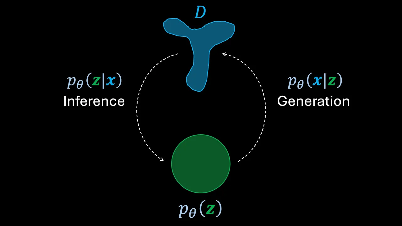








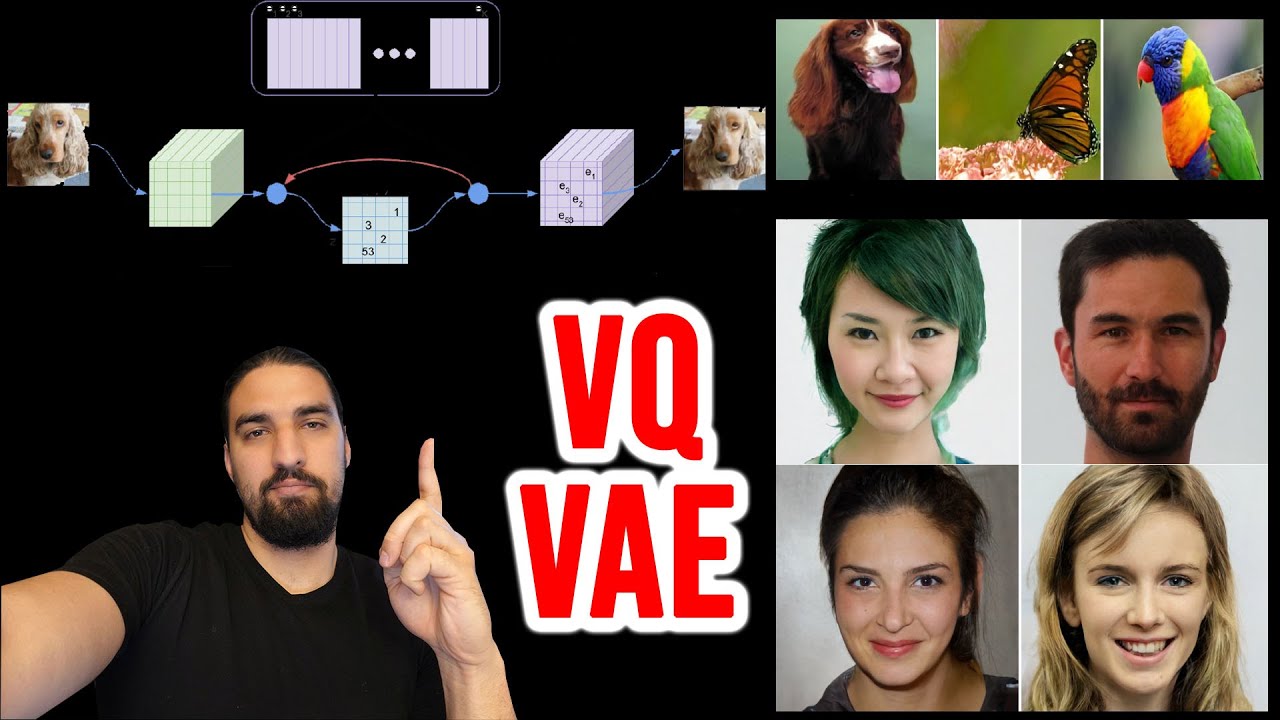





A Variational Autoencoder (VAE) is a type of unsupervised neural network that extends the basic autoencoder by learning a probability distribution over the latent space rather than producing fixed latent vectors, enabling it to generate new, varied image outputs instead of merely reconstructing training examples; the VAE architecture consists of an encoder that outputs mean and log variance for each data point, a reparameterization step that samples from this distribution to create the latent vector, and a decoder that reconstructs the image, with training involving both reconstruction loss (measuring how well the decoder recreates the input) and KL divergence loss (ensuring the learned distribution stays close to a standard normal prior).
Implementing Stable Diffusion VAE in PyTorch: A Step-by-Step Guide (50 chars)
Added:Proficiency in PyTorch, including constructing custom neural network modules, defining training loops, and utilizing autograd.
Fundamental concepts of standard Autoencoders (AEs), specifically encoder-decoder architectures, bottleneck layers, and reconstruction loss.
Theoretical understanding of Variational Autoencoders (VAEs), including the reparameterization trick, latent distribution modeling, and Kullback-Leibler (KL) divergence.
Deep learning for computer vision, specifically Convolutional Neural Networks (CNNs), residual blocks, and spatial downsampling/upsampling techniques.
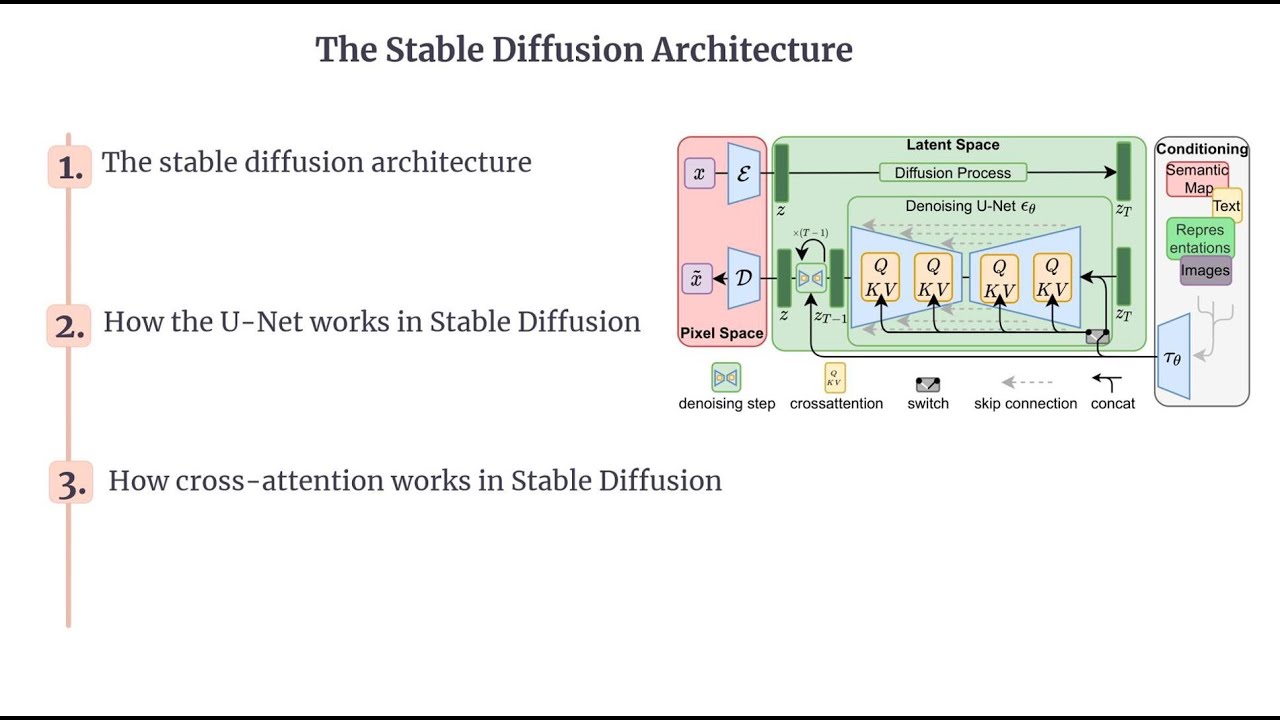
Integrating the implemented VAE into a complete Latent Diffusion Model (LDM) pipeline to enable latent-space denoising.
Studying the U-Net architecture and Cross-Attention mechanisms used to guide the diffusion process with text or image prompts.
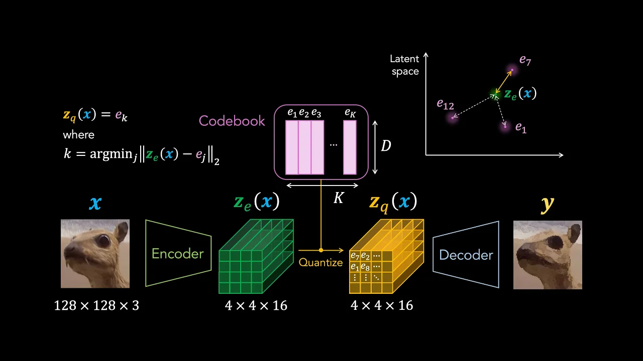
Exploring advanced latent representation techniques, such as Vector Quantized VAEs (VQ-VAEs) and VQ-GANs, to understand discrete autoencoding.
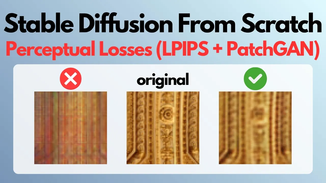
Implementing perceptual loss (e.g., LPIPS) and adversarial training (discriminators) to improve the visual fidelity of the VAE reconstructions.
31.1K views750likes43:18Original Release: 2024-12-04
Learn how to build a stable diffusion VAE from scratch using PyTorch. VAE stands for Variational Autoencoder. It's a type of autoencoder and a neural network that trains using an unsupervised technique. They're widely used in image generation models, mainly on latent diffusion-based and GANs-based image generation models. Machine learning engineer Harsh Bhatt teaches this course. Hey guys in this video we're going to learn how to implement VAE and train a VAE model. VAE is variational autoencoder which has huge impact in image generation model like stable diffusion and DALIN. Let's first take a look at like how VAE works and then we'll go to implement it and then train it. So to understand the VAE we need to first understand the autoencoder as it is the base of it. So autoencoder is an unsupervised learning neural network model. It is primarily used for dimensionality reduction so let's suppose if we want to train our stable diffusion models we cannot feed the 4k images to train the model which approaches like 8 million pixels to train the neural network which will be very computationally expensive. To solve this problem we will need a model which actually reduces the dimensionality of this 8 billion pixels into some fixed small vector with high rich features of those images. That's where the autoencoder comes in the picture which helps us to encode the image into a latent. So latent is a fixed point over the latent space so that's it our problem solved but that is not because autoencoder has some limitations when it comes to generations. So basically it is essentially designed to compress the images into latent and to reconstruct back to the original image so it lacks the ability to generate new and varied outputs. That's where the VAE comes into the picture unlike autoencoder rather than memorizing the patterns. It generates variations of images so the major technical improvement in VAE it does not directly generates the latent. First it generates the probability distribution and then converts it into the latent. So by learning and predicting the probability distribution over the latent space the VAE encodes each data points to not a fixed vector but as a range defined by mean and variance. So let's suppose if VAE is trained on 100 digits so the 7 will be in one pool and the 2 will be in another pool. So every digit have a unique pools in the latent space rather than a fixed vector or fixed point it will it will generate a pool of it and then as there are pools it has the possibility to generate the variations of it. But unlike in autoencoders where you have only a fixed vector for a specific thing and it is exactly based on what model has seen in the training examples. Suppose if we want to generate the number 7 it will going to generate the same close same as close to as the original one what has seen in the training images. The VAE actually learns this by predicting and learning the probability distribution and in the loss function it actually uses the reconstruction loss and the KL divergence which we're going to look at when we're going to implement this. So that's exactly what the VAE is and I hope you understood let's go and implement it. Hey guys so let's take a look at how to implement the VAE and then we're going to train it. So I have prepared a google colab notebook for you so we can run I can run the code at the same time and explain you how exactly it's working. In the VAE architecture you have this input image the input and then you have encoder which basically going to predict probability distribution view and it will give you this two things the standard deviation and the mean and then you can use this to create the latent space right and then you can use this latent space to reconstruct back using the decoder and then after decoding it you have the reconstructed image. Now to train this model you will go and do the backward pass and the loss will be for this is reconstruction loss plus KL divergence. So reconstruction as you already know about that the difference between the original image and the reconstructed image it could be like mean's gradual loss. So the KL divergence basically used to estimate the difference between two probability distribution.
So we add those two together and then it we have the final loss which we're going to use it to train it and so we'll have like a if you have millions of samples it will go in to train multiple times and then it will become much better. So as this is a very large model you can have like millions of images and it can able to generalize those very well. So first we have imported many modules which is not many actually but like some torches and maths functions a skid learn to have to train to split or NOS definitely. So I have written some like some explanation for you so let's suppose if you want to try together you I would recommend to try together and then you can or you can try it after and then read all the things like what exactly it is saying I have written some notes for you. So it's a good notebook to actually have to learn about VA which I will gonna use to if I need in future. So make sure you have this runtime D4 GPU so we're going to use GPU for this and then you need to run this I don't know why it's taking so long okay it's getting down.
So let's go ahead and then here we have I have explained about the self-attention self-attention you might probably know if not it's basically give you attention scores of different tokens if you have let's suppose in NLP natural language processing if you are like have sentences it just gives you the attention scores which features which tokens are more important sentence similar to in images or basically in visual models you have pixels so it will give you which pixels are most important give you the scores attention scores which will provide you the all the KQV scores and then you basically it has attention let me show you the attention scores so I think yeah this was a very bad image what the hell wow so attention of attention is all you need so I'm going to go to PDF one so ensure this all you need this will have very good information so yeah this is a formula this is formula actually which gives you the attention score and that's what it is describing here actually like the lines which are dim which has less attention scores which are very dark and bold which are actually have the highest attention score and it goes similar to pixels also right so here we are implementing self-attention self-attention are basically going to used with within the same sequence so let's suppose within the same pixels area so they are like cross attention also which I'm not gonna talk about here but self-attention is basically used for specifically same sequence so let's suppose if you have a sentence of something let's suppose I'm harsh so I'm harsh it will going to do it will divide into tokens of the same sequence and then match it each each other so I think it is actually in a self-attention because the law will never be perfect and the law will never be perfect matching the same tokens to each other right so that's what self-attention is so it goes against the same idea with the images so you have let's suppose you have to imagine they are like pixels and then the same pixel will be here and then to match and have a score of which each other right so that's that's so in init function we have self dot number of heads as we are like doing the same process of so in the init function we have number of heads in projection layer which is the linear layer which goes with dimension of like embedding dimension and three times of embedding dimension as we want to actually divide it into three tensors which like q, k, v you might already know about it so I would recommend to read this paper to understand about this self-attention it has like because it these three things which help us to attain the attention score q, k, and v right and this thing in the root it is the constant so now it's if you want bias is equal to in projection layer it's like true here and then our projection our projection is the output of this self-attention is the embedding dimension and embedding dimension and the bias will be based on the the argument right so and then we have self dot d heads which is like dimension of heads so the dimension of heads will be like the embedding dimension divided by the number of heads we have and the forward middle will have like this thing the x will be like a bad size sequence and dimension the bad size is something we will have this the sequence length in the images and images terms it will going to be the multiplication of the height and width so the let's suppose if we have three by five images that was 15 so 15 it will be the sequence length and dimension will be the number of channels of the images here so we are just extracting from this x the shapes and then we are defining interim shape which is the required shape we need to do to calculate the attention score in parallelly which is the back size sequence length and we are dividing to number of heads and the dimension of heads and then here we are getting we are calling the in projection layer and then we are chunking it out into three different tenses which has a shape of back size sequence length and d embedding which is dimension embedding and then we are changing it to the interim shape that is the required shape to do the to calculate the attention in parallel and then we are like transposing it to attain this shape which is this one earlier we had this um sequence length number of heads just we are like transposing it to just swap it out swap this thing so you had number of heads will come earlier and the sequence that will come later right um yeah so basically the back size number of heads and the the sequence line which is the heights and widths the multiplication of height and width and the number of channels you have you will have okay so now after that we can calculate the attention look to calculate the attention we have weight uh like the first part we are we are calculating the first part which is like q matrix multiply by k dot transpose by transposing it to actually do the to have the right shape for the matrix multiplication so after that if you want to fill mask of the weight then this code will actually do that and weights dot mask will fill the mask and then we have the weight divided by so it's the same formula which we have seen it here divided by dk right this is the same and then um and then the uh and then we are doing the f dot short max function so here we have the soft max and then the last we would multiply it with here we are multiplying it v and then transposing it back to the original one interim shape sequence length number of heads dimension divided by heads and then change back to the uh what it is required to have the output prediction this is bad size sequence length d embedding which was equals to what it has been uh during the what it how it came actually here and then we are using calling the out projection to get the output so that this is the all cell potential and the attention block is basically so this is all about the self-attention and then we have the attention block uh which just uses this self-attention in in the um residual p so basically you probably know about the residual we need to use a residual layers here because residual layers allow us to do the skip connection which help us to to create a deep network so if you don't have residual layer or don't do the skip connections there's a probability like not probability but yeah definitely the model going to be off it with few layers and uh we possibly can't train the very deep large models with large parameters so the large data will not able to generalize that work so this attention block uh so this initializes first group norm and the attention which is a self-attention module which we have defined and then forward we have this residual which we are used to loading the x first and then uh use uh calling grip norm and then then we are changing the shape to actually work with attention uh self-attention module here and then so basically as i describe we need bad size and then the sequence length and the channel so as in the input we have bad size channels and h in the blue rather than red so we are just uh you uh getting the features h multiplied by multiply by w so here i think we are doing it so we are changing the shape here uh x dot view would be like h multiplied by w so we will have just number of bad channels and h and w which is the features here and then we are transposing it so the h and w will become here and the channels so when we have the uh output from the attention we can just uh transpose it back and then in the last we are just adding the residual here uh which should be resistory here yeah yeah okay so um this was the attention block and then we can like i think i've called this one not okay and then i have to call this and then we have the visual block uh specifically for encoder and decoder so here uh i'm initializing the grip norm so normalization layer and then con one so in residual layer we don't actually change the shapes of the input so here also like we haven't changed the shapes in attention layer like the shapes were the same and also the output was the same output shape was the same so in the visual layer the the input and output shape will be the same also so the con one will actually extract the features but it will not change or reduce dimension as because the kernel size will be three and the padding one when the kernel size is three and the padding is one it don't change the shape i think there is formula for that you possibly can search it out to when when you apply con 2d there's a formula that based on in channels and out channels how much the um it reduces how much the shape is going to reduce or the the height width going to be reduced so this will not change the shape neither this one uh so there are two blocks here like the versus the con group norm and con one and group two no group two group norm two and con two right and if there's eight channels out channels are same just define the n and dot identity as a visual layer right so in forward function we have backside in channels and h and w and then we will just uh using the race issue here x dot clone and then dripped calling the group group norm and then there's a like activation function we are calling and the con one and then the second block which is the group norm two and the con two and then in the end we are adding the uh residual layer and x right so then we are moving forward to the encoder so encoder is um more interesting as it has more layers and like it going to actually do the mean work for us to convert into latents so this whole class is basically sequential here so directly defining this in our super dot init and so first we have this con 2d to actually so basically the intention for it is going to be here so so we will basically reduce the dimensions from here so you're going to see a lot of con 2d layers and so the first we have the con 2d layers which actually i've also defined here the shapes like the what was the initial shape and how it going to impact and like what exactly the output shape going to be so here we're not changing the um size of the image but just the channels and then we have um residual block uh so we were going to use more various so we were going to use lot of residual block in between because we need to have a very deep network so we're going to use residual block uh a lot here between the con 2d so then we have another con 2d and then here we have stride 2 so which um has h divided by 2 divided by 2 so half the size of the image now we have and again residual block, residual block and con 2d now we have the divided by 4 size and then we have residual block, residual block so it's kind of same pattern you have till we do this until here until we reach the h divided by 8 like until we reach x divided by 8 w divided by 8 and then uh we can just use the attention block here for doing the attention stuff and then again we uh in the end we have just uh we we can use residual block and then and in the end block of it uh we are using residual block and the group normalization and this uh salu function activation functions and this con 2d layers so the final uh shape will be going to be bad size 8 channels h divided by 8 and w divided by 8 so so we have reduced the size of the image very much and then we can use it to generate the latency and then decode it back in our forward function first we are doing is uh we are padding it so x equals to f dot pad so it going to pad it uh to the right and bottom and then after that we are chunking it the mean and variance which is the more most important part of the va initial uh most important part of the va initial size we had bad size 8 s divided by 8 w divided by 8 and then we are generating the not generating but like chunking it into two tensors which is uh bad size and then we have like four dimensions because we are uh we are chunking it in dimension one so this is going to be half the channel is going to be half so yeah from eight to four and this will going to be the same so mean and log will have the same inner dimensions which like uh h divided by 8 and w divided by 8 and then um then we are doing is we are doing log so this is the log variance so it's not the variance log variance which we going to use to clamp and then we are doing the re-parameterization technique which is uh the process of generating the latent so how we doing is this is the std standard deviation so we you we can use the log variance and then call this dodge dot exponent function to have the to generate the standard deviation and then this eps is basically uh the eps is something i think um wait what is eps yeah i think eps is basically the um so eps is uh so oh oh so eps is uh the constant so it's like dodge or trend line and then this is the formula for the uh generating the latent so the x is our latent which we can also say it like a z and then we are just multiplying with some constant which this constant is coming from like a artificial library uh and in the decoder we can we will going to divide it also this constant so this was all about the encoder and uh now let's take a look at decoder so in decoder we have again this uh so the intention let's take a look at what are the intentions so now we have the latent space the intention for the intention to use the decoder is to actually use this latent space to reconstruct back the original image that's what the decoder uh is going to do so again it's a sequential layer it's going to uh it has various residual layers and contour d layers the main layer in here is upsample so so nn dot upsample which going to upsample by a factor so here it was earlier we had like bath size for 32 by 32 image and then when we're going to call this uh function we're going to upsample it by a factor of 2 because the scale factor is 2 so it's going to be 64 city floor and then we are calling it uh at a certain interval after defining contour d and a screw block and then here we the same scale factor which is 2 we have 128 and then we're going to do this again to buy 256 because our uh input image going to be 256 and output image going to be 256 so and then we actually again using the group norm and then nn dot value activation function uh in forward method first we actually removing the constant what we have multiplied it with x and then we just like iterating it all the models we have in the decoder and we are returning this x which is the output so the output will be going to be the shape will be going to bath size three will be the channel so the the original image in uh channel and the original image height original image at width we are going to return it so that was the decoder and then we can call it i think i haven't called this encoder yet call this one oops encoder and decoder so yeah so this was all about the um va and uh now we can like use these modules to actually train the va so the next part is to download the process data so i have so i already have this data set of docs it consists of images of dogs of various uh breeds and then you have this you can unzip it and here this function we're going to split it into the training and test dir and this class this this is the last model which wraps all the encoder and decoder so we can call this and then the last uh cell we have is and then we have like a train va so here we are basically uh using this va module to actually create a training loop and then to do the back forward and backward pass so let's take a look at what are the constants and how we are defining it so the number of people going to be 100 just like you can tweak it up like to certain level and how much you can train uh learning rate learning rate is like one this is the learning rate is like a typical learning rate for va which i think probably it can converge it better with that but you can tweak it if you want to and then we have beta which is like kl divergence weight so as i mentioned kl divergence is like is used to find a difference or integrate the for the comparison up to uh probability distribution so here we will use this uh in the kl divergence loss this will transform to a specific shape and the transform transforms dot compose function that size will have four you can just tweak it up uh based on your memory uses and um data set uh this this defines data sets and then it's a data loader we are defining data loader from here and then here we have a model using the va module and then the optimizer we're going to be the adam one yeah and then here we have learning it also we are like um using accumulation of step so we have here yeah yeah we are just using accumulation of steps if you don't know about the accumulation of steps i would recommend to a little bit read about it like how this works accumulation of steps it's basically like normalize the loss to account for accumulation so all the like the and here just we are storing the training losses uh so in our training this is our training loop uh now we can train our v now finally okay so just model a train typical thing and then here the and then here we are iterating over the data loader image that uh putting into a device i think device we have what was yeah good advice so and then forward pass it will return deconstructor encoded model so as the model is v which returns the two things decoded and encoded right so so reconstructive which is like a decoder and encoded the latent vector and now we need to compute the loss the reconstruction law is going to be msc loss uh which going to be reconstructed and b compares it with images the original image then extract mean and log variance from the encoded so as we have already mentioned it so so we had the latent so now we are again uh yeah again extracting it mean and log variance uh although like i think you can try it up with uh not again uh splitting up like in so i think here i'm like uh first chucking it into mean and log and then defining it again i think that's the right way to do it i believe and then again i'm uh extracting the mean and log variance but let me know if you read or like uh know that we can do any other way based on what i know we can extract uh again mean and log variance and then use it over the KL divergence laws to calculate the KL divergence so this formula calculates the KL divergence i think you can read more about the KL divergence already formula so so this is the formula actually um so you can you can read more about it possibly uh so this KL divergence we will going to use it uh as it was mentioned here reconstruction plus KL divergence so so the total loss will be equals to reconstruction plus the KL divergence so we are like multiplying with the constant the KL divergence we're going to have a constant multiplied which we have to find here the beta now we have a loss and then now we can do the backward pass here and uh this to the uh optimize.zero grad dot step optimize.step and zero grad and storing the training losses of um this basically i'm just i wanted to see like reconstructed image so at every step i'm like generating this uh reconstructed image reconstructed.py which you can actually try it out during the training you can just uh at every step it will save the image so you can check it out like how what how exactly the eating constructor image looks like uh so i think let's call this and let's see how exactly this is training and then we can check it out the constructed.py dng yep so it started training and yeah and then this is the constructed.png looks like a very small image but i think yeah initially you probably won't able to see anything um but after like training at a certain level you possibly can see the dog which is here so that was the all about the VAE the instrumentation and how to train it hey guys so this is a second part of the video of building and training VAE uh so uh in that video i explained how to build a VAE from scratch and how to create a training pipeline of it and train it so in this video i have trained a VAE uh till 19th epoch so this is my trained model file what i'm gonna do with this is i will gonna use our custom VAE like the VAE we have implemented uh here like the this VAE uh the model we have implemented all the things in core and decoder and attention block and decision block we will going to integrate this into the stable diffusion pipeline and then we will try to generate an image with that that's why i have trained this VAE till 19th epoch which is still very early and uh still not very generalized but it gonna work in the way where we can just recognize whatever we are prompting uh so let's try this um class VAE so this is the our older VAE section but uh for that making compatible with diffusion library and diffusion stable diffusion pipeline to create our custom VAE which has some specific functions so this is a custom VAE and then this encode function this decode function and the forward function will just only return the x reconstructed z is the latent from the encode uh from the encoder and the x reconstructed is the image we have from the decoder this load pre-trained weights will going to load the state dict of the this model which we're gonna use and then we have another module which is a diffuser comparable VAE here we are uh loading uh autoencoder kl which is like a another module torch module which help us to create comparable VAE uh with like diffuser comparable VAE so i'm using her as an inheritance so this diffusion comparable we have all the functionality what autoencoder kl has here i'm just defining cell.va to VAE um and getting the VAE from the constructor and then the encode and decode function uh here some of the things i'm printing just like debug and stuff like that so yeah i think just run this thing and then run this thing and then here i'm uh loading the uh this compvist class table diffusion you can just like i can go here show you what kind of model this is this is a stable diffusion model yeah oh it was released on i think 2022 and uh plus yeah i think this model will work with our VAE it is a 512 by 512 model by running this you can download this in the local DIA here uh dot slash model DIA and then the next you have to do is like you have to uh just check it out like what exactly uh the base structure of it and i have basically tried to look at it okay what other things it has and what other things i need uh to be made compatible like whatever the VAE we have constructor implemented how to make compatible with that autoencoder klva so the next we have is like i'm just importing a torch here i'm loading the our strained custom VAE uh which is like here VAE model repop 19.pth file this is a pts file my application is CPU so in this section i am replacing some typos and stuff so because like there were some missing keys and stuff like that so and it was not very compatible like the our implementation was not compatible to the what we wanted to actually do with uh stable diffusion so i have to actually replace some namings and stuff all the way like the architecture is is same but the namings and stuff is different that's why i'm using this uh which this code will actually replace some names and stuff but the architecture going to be the same and it will add all the uh keys and stuff there right um so this is what it does and then just it just loads the VAE then i can just we can just see uh the architecture of the VAE here and you can just check it out like how it is constructed and match it out like the other VAEs or basically you can load other VAEs like i'm loading this one right now this um a diffusion model you can try to load another diffusion model uh possibly like it should be like 512 by 512 because if we go with STXL something different uh bigger models it won't work so yep and then what we are doing is like we are just loading the stable diffusion pipeline this VAE custom VAE comparable VAE and then inside this we are just putting the VAE and then here stable diffusion pipeline dot from pre-trained the stable diffusion model and the here we have the option to uh integrate the custom VAE or whatever the VAE want to integrate so this is here we are just injecting the comparable VAE and then pi dot 2 and moving to CUDA let's run this and here prompt is our photo of a dog and then the we are running the pipeline with inference step is 50 let's see how this image will look like i'm using this promo photo for dog because our VAE is trained on the dog photos so let's see okay so it does uh look like a dog like you can just recognize it although like the image quality is like very noisy because the VAE is trained uh till only 19 epoch it should like go to like 100 epoch or something like that and like originally VAE is trained till like a huge number of hours uh so we haven't trained that much uh i don't have that much compute at the moment to actually train that but if you want to try please try it and then try to integrate that VAE and then try to see how the image quality is improving and let me know guys how this will work if you want to try this out but that's it for the for this tutorial i hope you enjoyed and understood let me know if you have a question and if you want to see more content like this tutorials subscribe to coded harsh thank you guys for watching this video yeah
Up Next

37:20
AI Diffusion Models: How Text Becomes Images
@3blue1brown
1.5M views•2025-07-25

57:48
Secure Multiparty Computation (MPC): Foundations & Challenges
@SimonsInstitute
7.3K views•2015-05-28
27:51
Machine Learning and AI Concepts Explained with Animations
@freecodecamp
241.3K views•2025-04-22

18:41
Neural Networks Explained: Math, Layers, and Learning Fundamentals
@3blue1brown
21.9M views•2017-10-05
Related Study Plans & Knowledge Roadmaps
Structured learning paths in Artificial Intelligence
artificial-intelligence
Aligning LLMs: DPO, TRL & Custom Datasets
01Foundations of Python & Machine Learning
02Transformers and Large Language Models (LLMs)
03Aligning LLMs: SFT and RLHF
+ 3 more learning modules
24h6 modules
Explore Roadmap
artificial-intelligence
Federated Learning: PyTorch, Flower & Privacy
01Python & Machine Learning Foundations
02Deep Learning Basics with PyTorch
03Introduction to Federated Learning
+ 2 more learning modules
35h5 modules
Explore Roadmap
artificial-intelligence
Securing LLMs: Guardrails AI & NeMo Gateway
01Introduction to LLMs, Python, and APIs
02Understanding LLM Vulnerabilities & Threats
03Defending LLMs with Guardrails AI
+ 2 more learning modules
15h5 modules
Explore Roadmap
artificial-intelligence
Building Recommenders: Two-Tower & Vector DBs
01Foundations of Python & Machine Learning Basics
02Introduction to Recommender Systems
03Deep Learning & Representation Learning
+ 3 more learning modules
75h6 modules
Explore Roadmap