Latent Diffusion Models Explained: How Stable Diffusion Works

[00:00:00]Hey, have you been on Twitter during the  last weeks? Or were you on Holidays, like me?

[00:00:06]Because if you were on Twitter, there is  zero chance that you weren’t hit by somebody posting about Stable Diffusion,  just look at all of this!!

[00:00:17]What is Stable Diffusion,  you ask from your hammock?

[00:00:21]Well, Stable Diffusion is an  open-source alternative to DALL-E 2.

[00:00:25]So unlike DALL-E 2, which is  hidden behind an API and a paywall, Stable Diffusion is a text-to-image generator  like DALL-E that has open-sourced its code, then the weights for academic purposes, and as of very recently, it has even  released the model weights for everyone!

[00:00:47]Today, we explain Latent Diffusion Models which is  the algorithm that stands behind Stable Diffusion.

[00:00:55]And Latent Diffusion Models, or short LDMs,  are a special kind of the more general class of diffusion models about which you  may or may not have heard already.

[00:01:08]So, if you are interested in how Stable Diffusion  works, this might be just the right video for you!

[00:01:14]But before we dive into the explanations, let’s  thank AssemblyAI for sponsoring today’s video!

[00:01:21]Do you know that feeling when you  have hours and hours of audio data lying around and you want to  transcribe it – automatically?

[00:01:28]Yes, I do know that feeling, especially because I do not want to enter  the captions manually for every video I do.

[00:01:35]Luckily AssemblyAI, can help me transcribe my audio with state-of-the-art APIs  for automatic speech recognition!

[00:01:42]And you can use their APIs too, to  automatically convert recorded audio.

[00:01:48]But wait, there is more! You  can even transcribe in real-time live audio streams into text, which can come  in handy for conferences or other live streams.

[00:01:58]And believe me that AssemblyAIs models do not stop  there: it can even help you understand your audio data, for example it can summarize the content  and detect the topic of what is being said.

[00:02:12]Or it can automatically tag bad words,  if one happens to slip out. So, what are you waiting for, check out AssemblyAI  with the link in the description below!

[00:02:22]I for example, used AssemblyAI to  transcribe my speech for this spot, and you can see in the subtitles how well  it works. And think about it, I am quite a hard example for speech transcription,  with my Eastern European accent.;) Now back to the video! First, let’s  recap what diffusion models are.

[00:02:42]For more details for example on classifier-free  guidance, do check out our previous videos on this. But, as far as our explanations  of diffusion models in general go, this video has the technically  most correct version, because we cleared up a confusion that  Ms. Coffee Bean had this whole time.

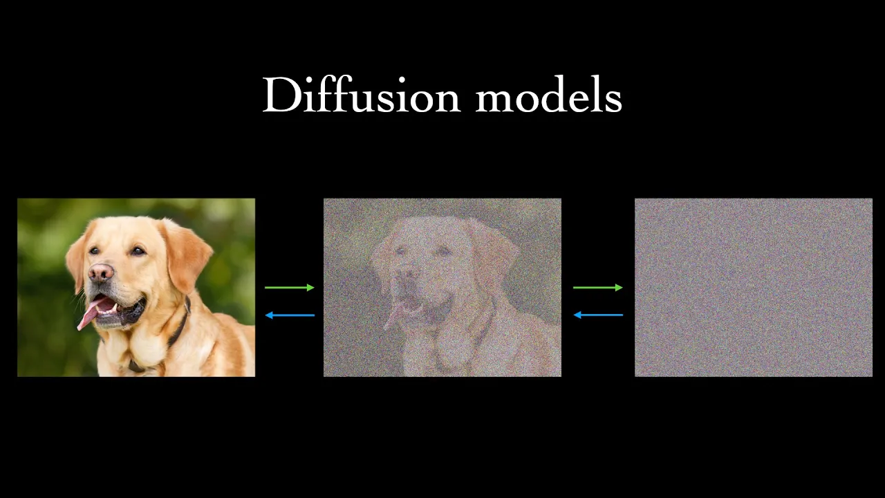
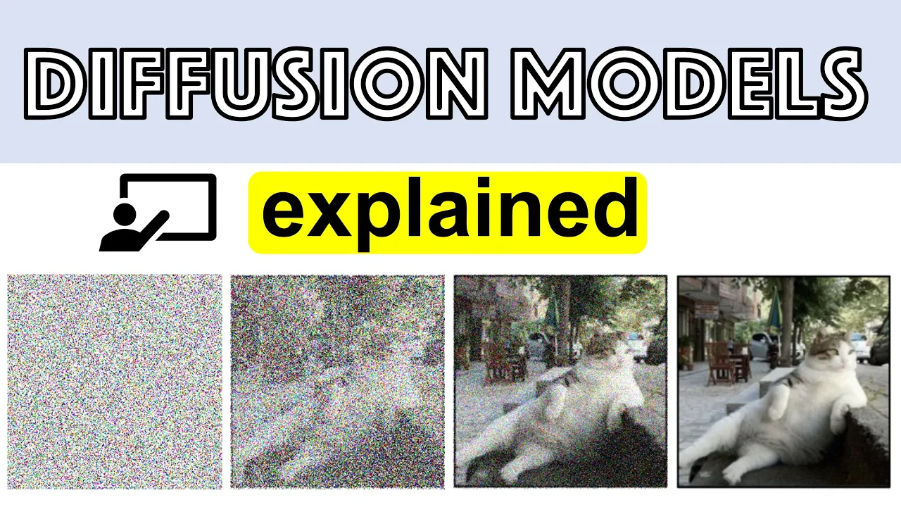
[00:03:03]But let’s not get ahead of ourselves and  talk about diffusion models first! The diffusion process is where you diffuse  more and more noise into your image.

[00:03:14]So, you take an image, and in t steps,  you gradually add more noise to it, until at the last timestep t, the  image is approximately just noise.

[00:03:26]Diffusion models go in the opposite direction, in other words, they learn to  reverse the diffusion process.

[00:03:35]When we are trying to generate  an image with a diffusion model, we follow each of these t steps and  reduce the noise gradually, step by step.

[00:03:44]For this, we use the same neural network,  so just one neural network, usually a U-Net, to go from step t to step t-1 and here,  for visualization purposes we have chosen step t to be a noisy dog and step t-1  to be a less noisy version of the dog.

[00:04:04]Short sidenote on U-Nets: A UNet is a  convolution-based neural network that is downsampling an image into a lower dimensional  representation and reconstructs it during upsampling. The downsampling and upsampling stacks  of layers communicate through skip connections.

[00:04:25]And now, what exactly is the  input to the neural network?

[00:04:30]It’s an image at step t and the neural  network’s output is the total noise that should be subtracted from the  noisy version of the image at step t to reconstruct the original image,  so the clear picture of the dog.

[00:04:48]Wait, let’s untangle this a bit and  recapitulate the whole diffusion thing from the beginning because it is an important  detail Ms. Coffee Bean got wrong so far (of course, I knew the  correct version all the time).

[00:05:01]Unfortunately, the papers are not so clear about  it. How it is done becomes clear from the code.

[00:05:07]The diffusion process is all about going from  a little noise to more noise. The backward diffusion process is the reverse, and this is  what we do with the help of diffusion models.

[00:05:20]And the diffusion model itself, so this  one U-Net that we apply at each step, gets a noisy image at step t and predicts  the whole noise that the image contains, and not just the noise we need  to subtract to get from t to t-1.

[00:05:36]It’s just that we do not trust the model enough  to just subtract this whole noise in one go, so at each step, we extract just a fraction of  the total noise from the image at timestep t.

[00:05:48]Reasons for going step by step is  that we break down a hard problem, of generating an image from just noise, into t steps, where each step can correct and  improve upon the previous one, especially when the whole time we are trying to inject textual  information when doing text-to-image generation.

[00:06:07]It's easier to inject textual  information gradually than all at once.

[00:06:12]Ok, so this was basically an  erratum to our previous videos, where we thought that at each step, the  model predicts only a fraction of the noise.

[00:06:21]But actually, the diffusion model predicts  the total amount of noise from which we then subtract only a fraction to give it  afterwards yet another go at denoising.

[00:06:32]But now, how does the text come into play? It  is injected into the whole process in two ways: First as input to the diffusion  model by concatenating the text representation coming from a language  transformer to the image input.

[00:06:47]And second, through cross-attention, letting the  U-Net attention layers attend to the text tokens.

[00:06:54]Now, what about Stable Diffusion,  and how does this work?

[00:06:57]The idea behind stable diffusion was  introduced in this CVPR paper called “High-Resolution Image Synthesis  with Latent Diffusion Models” from Heidelberg folk [proud]  who now moved to Munich [sad].

[00:07:11]The authors proposed latent diffusion models, or short LDMs, to address a  shortcoming of diffusion models: When trying to generate a large image, such as a 1024 x 1024 image, then the U-Net in here, would have to take  in a 1024 x 1024-dimensional noise grid and produce an image out of it.

[00:07:33]As you can imagine, this can become  really expensive for one diffusion step and one has to do it t times,  where t can be something like 150.

[00:07:42]What people did so far to circumvent  this high dimensionality problem, as we have seen in the GLIDE paper for example, is that they actually train their diffusion  model on much smaller images, like 256 x 256 and then have an extra neural network  that learned to upsample and sharpen 256 x 256 to higher resolution, for  example. And this is one way to do it.

[00:08:08]But LDMs take another approach. The core concept of LDMs is to surrender the idea of working in the image  space and work on a latent space instead.

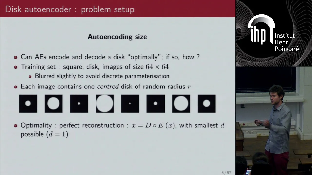
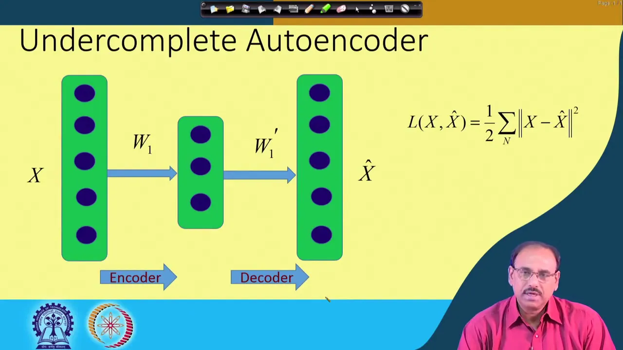
[00:08:19]You may think of it as of an autoencoder  encompassing the diffusion model, as follows: For diffusion models, we had the original image  to which we added more and more noise. But now, we do not work with the image itself, but with a  lower-dimensional representation of it, because we take the image and run it through an  encoder, which is basically a VQ-VAE.

[00:08:40]This encoder also has a decoder  to reconstruct the image.

[00:08:44]This encoder and decoder  are trained together first, to encode the image into a lower dimensional  space and then reconstruct the image from it.

[00:08:52]Now, instead of applying noise onto  the image for the diffusion step, we apply noise onto the lower-dimensional  representation of the data.

[00:09:01]And for the backward diffusion, the  U-Net works with this representation instead of the whole image. Since the  image representation is lower dimensional, the U-Net does not have a  lot of heavy lifting to do.

[00:09:14]Even more, by compressing the image first through  the encoder, the encoder decoder can take care of image details and let the diffusion model  focus on the important image semantics.

[00:09:28]This makes LDMs much faster than usual  diffusion models, so this enables us to run Stable Diffusion on laptop hardware, instead  of clusters or you know, OpenAI servers! 😉 We hope you see how clever, but similar  LDMs are to what previous work like GLIDE did: GLIDE, took an image, downsampled  it from let’s say, 1024 x 1024 pixels to 256 x 256 resolution with a usual image  downsampling algorithm, staying in image space.

[00:09:58]Then they ran diffusion and upsampled the  result to get a high-resolution image.

[00:10:04]Now with LDMs, instead of a standard downsampling  algorithm that produces low-resolution images, the LDM encoder takes a high-resolution image  and embeds it into a compressed code of its own, that captures the semantics of the  image, but in a space that does not look to us like the original image anymore.  And the diffusion model can take it from there.

[00:10:27]As you can see from the paper, the author’s  initial work on LDMs was producing images of human faces and objects. This is because  the model whose output we see in Figure 1, was trained on human faces and objects.

[00:10:40]And you know, what kind of data comes into the  diffusion model, this is what they also produce.

[00:10:45]What makes Stable Diffusion so special and fit  for art generation, is that it was actually an LDM trained on a core dataset consisting of, we cite  “LAION-Aesthetics, a soon to be released subset of LAION 5B. LAION-Aesthetics was created with a new  CLIP-based model that filtered LAION-5B based on how “beautiful” an image was, building on ratings  from the alpha testers of Stable Diffusion”.

[00:11:15]And this different training data makes  it have its own style that is different from other text-to-image generators  like DALL-E 2, Midjourney or Imagen.

[00:11:23]So to sum up: what is now Stable Diffusion?

[00:11:26]It is basically the work that follows  the Latent Diffusion Models paper, where authors of the paper teamed with StabilityAI  and communities such as Eleuther AI and LAION.

[00:11:37]Now, with Stable Diffusion we have an  image generator tuned to produce art, as it was trained on “beautiful” images,  which were often produced by human artists.

[00:11:48]It will be interesting to see what kind of new  copyright law these AI generations will spawn.

[00:11:54]Some artists feel bad to see that AI can now  do something in seconds that took them hours to make. But other artists consider the AI to be  a sort of tool, which still needs human input.

[00:12:07]And the human hours that go into diffusion-based  image generation is not a neglectable amount.

[00:12:14]Just think about the hours one can spend  in tuning the text prompt and waiting for the right result to come out, only to notice  that the astronaut is riding the horse again, when I actually wanted the horse  riding the astronaut on the moon!

[00:12:28]If you are interested in using Stable Diffusion  yourself, then check out the diffusers library or any other helpful tutorials out there.

[00:12:36]It’s really amazing what the community  has put out in such a short amount of time in terms of documentation and in terms of generations.

[00:12:45]Just look at this Twitter user bringing  their 4 year-old’s sketches to life.

[00:12:50]Wow. Do you think this is creativity?

[00:12:53]We’re so curious to know what you think about this so, we’ll be watching the comment section closely.

[00:12:59]Ms. Coffee Bean, it is time to say  goodbye. See you in the next video!

[00:13:05]Okay, bye!