
![[딥러닝의 기초] 250923 Chapter 3(2): Backpropagation, and Depth vs. Width of DL](https://i.ytimg.com/vi/uLO8K9qLMRU/maxresdefault.jpg)






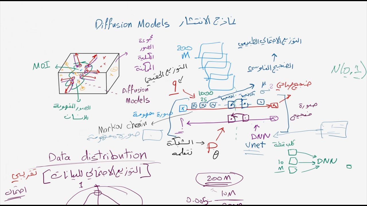













Stable Diffusion is a generative model that creates images by iteratively removing noise from random noise using a U-Net architecture trained to predict noise levels, combined with CLIP encoders that translate text prompts into embeddings to guide the image generation process; the model works by starting with random noise and applying multiple denoising steps where each step predicts and subtracts noise based on both the current noisy state and the text embedding, ultimately producing an image that matches the prompt description.
Deep Learning Foundations to Stable Diffusion | Lesson 9 (2022)
Added:Fundamental concepts of Deep Learning, including neural network architectures, backpropagation, and loss functions.
Basic understanding of Autoencoders and variational inference principles, particularly how images are compressed and reconstructed.
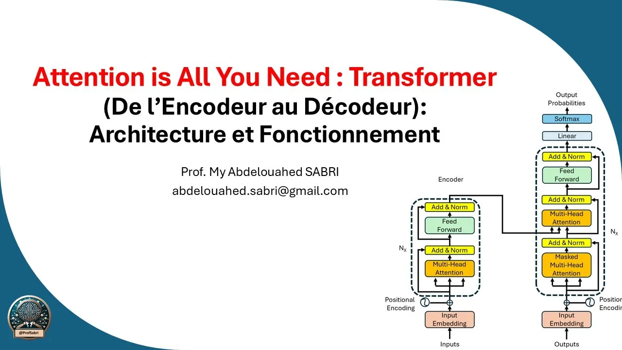
Familiarity with the Transformer architecture and the concept of attention mechanisms, which underpin text encoders like CLIP.
An introductory understanding of probability theory, specifically Gaussian noise and Markov chains, which form the mathematical basis of diffusion.
Practical implementation of fine-tuning techniques for diffusion models, such as LoRA (Low-Rank Adaptation) and DreamBooth.
Advanced conditioning methods for image generation, specifically exploring ControlNet and T2I-Adapter architectures.
Investigation of different sampling schedulers (e.g., DDIM, Euler, DPM-Solver) and their mathematical impact on generation speed and quality.
Exploring the application of diffusion models to other modalities, such as video generation (Text-to-Video) and 3D asset creation.
171.7K views2.6Klikes2:15:15Original Release: 2022-10-20
Lesson 9: Deep Learning Foundations to Stable Diffusion, 2022 https://youtu.be/ZkOtBv123V0 Hi everybody and welcome to “Deep Learning Foundations to Stable Diffusion”. Hopefully it's not too confusing that this is described here as Lesson 9, that's because strictly speaking we treat this as Part 2 of the “Practical Deep Learning for Coders” series.
So that Part 1 had eight lessons so this is lesson nine. But don't worry you didn't miss anything, it's the first lesson of Part 2, which is called “Deep Learning Foundations to Stable Diffusion” and maybe rather than calling it “Practical Deep Learning for Coders” we should call this “Impractical Deep Learning for Coders” in the sense that we are certainly not going to be spending all of our time seeing exactly how to do important things with with deep learning.
But we'll be doing a whole lot of fun things —generative modely fun things— and also a whole lot of understanding lots of details which you won't necessarily need to know to use this stuff but, if you want to become a researcher or if you want to, like, put something in production —which has got like some kind of complex customization requirements, stuff like that, then it is going to be very helpful to learn the details we'll be talking about.
So here in Lesson 9, there's kind of going to be two parts to it. One is just a quick run through —quickish run through of using Stable Diffusion— Because we're all dying to play with it, right? And then the other thing that I'll be doing is describing in some detail what's going on, how is it working.
There'll be a whole lot of hand waving, either way, because it's going to take us a few lessons to describe everything from scratch but hopefully, you know, you'll get a, you'll feel like you'll come away from this, with this lesson with a reasonable, you know, intuitive understanding, at least, of how how this is all working.
Assumptions. Well, I'm going to try to explain everything, like, everything. I'm going to try to explain everything so, like, if you haven't done Deep Learning before this is going to be very hard but I will at least be trying to say like, this is roughly what's going on and where you can find out more.
Having said that, I would strongly suggest doing Part 1 before doing this course unless you really want to throw yourself in the deep, deep end and give yourself quite, quite a test.
If you haven't done Part 1 of “Practical Deep Learning for Coders”. But you're, you know, reasonably comfortable with Deep Learning basics, you could like, write a basic SGD loop in Python.
And you know, you know, how to use, ideally Pytorch —but Tensorflow is probably okay as well.
And you kind of know the basic ideas of how to create, you know, what an embedding is and you could create one of those from scratch, stuff like that, you know, you'll probably be fine.
Generally speaking, for these courses, I find most people tend to watch the videos a few times and often the second time through folks will like pause and look things up they don't know and check things out. Generally speaking, you know, we expect people to be spending about 10 hours of work on each video. Having said that some people spend a hell of a lot more and go very deep, some people will spend a whole year, you know, sabbatical studying “Practical Deep Learning for Coders” in order to really fully understand everything so really it's up to you as to how deep you go.
Okay, so, with that said, let's jump into it. As I said the first part we're going to be playing around with Stable Diffusion and I, you know, try to, you know, prepare this as late as possible so it wouldn't be out of date.
Unfortunately, as of 12 hours ago, it is now out of date, and this is one of the big issues with the bit I'm about to describe which is like: how to play with Stable Diffusion, exactly how do the details work. Which is, it's moving so quickly that all of the details I'm going to describe to you today and all of the software I'm going to show you today, by the time you watch this, if you're watching it —so what is it we're up to now, it's 11th of October— so if you're watching this in, like, December of 2022, or watching this in 2023, the details will have changed. So what's happened today in the last 24 hours is: two papers have come out so what I was going to be telling you today is for example to do a Stable Diffusion generative model the number of steps required has gone down from a thousand to about 40 or 50, but then as of, yeah, last night, papers just come out that's saying it's now down to 4, that is, 256 times faster. And another paper has come out with a separate —I think— orthogonal approach, which makes it another, let's see, 10 to 20 times faster.
So things are very exciting. Things are moving very quickly. Now, having said that, don't worry because after this lesson we're going to be going from the foundations —which means we're going to be learning all the things of how these are built up— and those don't change much at all. And in fact a lot of what we'll be seeing is extremely similar to another course we did in 2019, because the foundations don't change and once you know the foundations these kinds of details about the stuff that you'll find in these papers, you'll be like: “oh, I see, they did all these things the same way as usual and they made this little change”. So that's why we do things from the foundations, so that you can keep up with the research, do your own research by taking advantage of this foundational knowledge which, you know, all these papers are building on top of.
So anyway, I guess I should apologize that even as I record this, you know, the notebook is now one day out of date.
So in Part 1, you know, you might remember we saw this stuff of Dall-e 2 illustrations of Twitter, by Twitter bios, which really are pretty cool.
So, you know, the cool thing is that we're now at a point we can build this stuff ourselves, and run this stuff ourselves. We won't actually be using this particular model Dall-e 2, we’ll be using a different model: Stable Diffusion. But has very similar kind of outputs. But we can go even further now, so, one of our wonderful alumni, Alon, actually recently started a new company called —I don't know who said— it's strumer (strmr.com) where you can use something that we'll be learning about today, called Dreambooth, to put any object, person, whatever into an image.
And so he was kind enough to do a quick Dreambooth run for me and added these various pictures of me using his service. So here's a fun service you can try. One crazy one he tried was me as a dwarf which, I gotta say, actually worked pretty well. This half looks like me, I reckon, and then the bottom bit is the dwarf version. So thank you a lot and congratulations on your great progress since completing the fastai course. Yeah, I love it.
So, something that's a bit different about this compared to previous courses —a lot of previous courses— is this is no longer just a me thing because this is moving so quickly I've needed to get a lot of help to even vaguely get up at the gate and stay up to date.
So everything I'll be showing you today is very heavily influenced by extremely high levels of input from these amazing folks —all of whom are fast AI alumni.
So Jonathan Whitaker —who I saw in our chat— is, was basically the first guy to create detailed educational material about Stable Diffusion and has been in the generative model space, well, for a long time by Stable Diffusiony standards —I guess.
So Wasim um has been an extraordinary contributor to all-things fastai.
Petro came to San Francisco for the last time we did a Part 2 course in 2019 and took what he learned there and made his amazing Camera+ software dramatically better and had it highlighted by Apple for the extraordinary Machine Learning stuff added and he's now at Hugging Face working on the software that we'll be using a lot —diffusers— and then Tanishq —everybody in the forum of the fastai community probably already knows— now at Stability.Ai working on Stable Diffusion models, his expertise particularly as in medical applications.
So really folks from all the key groups —pretty much— around Stable Diffusion and stuff are working on this together. And you'll also find some of these folks have recorded additional videos going into more detail about some of the areas which you'll find on the, on the course website. So make sure you go to course.fast.ai to get all the information about, you know, all the materials that you need to take full advantage of this. So every lesson has links to notebooks and to details and so forth. If you want to go even deeper, head over to forums.fast.ai, enter the Part 2 2022 category, hit on the “about the course” button and you'll find that every lesson there's a chat with even more stuff. So look at this carefully to see all the things that me and the community have provided to you to help you understand this video and also check out the questions underneath and answers underneath to see what people have talked about. They can get a bit overwhelming so once they get big enough they'll, you'll see that there's a summarize button that you can, that you can click to kind of see just the most liked parts. So that can be very helpful.
Okay so, they're all important resources, I think, to get the most, to get the most out of this course.
Now, compute, so I'm completing Part 2 requires quite a bit more compute than Part 1.
Compute options are changing rapidly and, to be honest, the main reason for that is because of the huge popularity of Stable Diffusion. Everybody is taken to using Colab for Stable Diffusion and Colab's response has been to start charging by the hour for most usage. So you may well find if you're a Colab user —we still love Colab. You may find that, you know, you run out of, they start not giving you decent GPUs anymore and if you want to then upgrade, they limit quite a lot how many hours you can use. So at the moment, yeah, still try Colab, they're pretty good, I mean, for free you get some decent stuff, but I would strongly suggest trying out also Paperspace Gradient. You can pay like nine dollars a month to actually get some pretty good GPUs there at the moment.
Or I'll pay them a bit more to get even better ones. Again, but the thing is this is all going to change a lot, I don't know, like, maybe people will make Paperspace Gradient have to change their pricing too, I don't know, so check course.fast.ai to find out what our current recommendations are.
Now, Lambda Labs and Jarvis Labs are also both good options. Jarvis was created by alum of the course and has some just really fantastic options at a very reasonable price. And a lot of fastai students use them and love them. And also check out Lambda Labs who are the most recent provider on this page and they are rapidly adding new features. But the reason I particularly wanted to mention them is, at least as I say this, which as I say is early October 2022, they're the cheapest provider of kind of big GPUs that you might want to use to run like serious models. So they're absolutely, yeah, well worth checking out. But as I say, this could all have changed by the time you watch this, so go and check out course.fast.ai.
Also, at the moment: late 2022, GPU prices have come down a lot and you may well want to consider buying your own machine at this point.
Okay so what we're now going to do is jump into the notebooks and so there's a repo that we've linked to called “diffusion-nbs” which isn't kind of the main course notebooks —it's not the “From the Foundations Notebooks…”— there's just a couple of notebooks that you might want to play with, a bit of fun stuff to try out. One of the interesting things here is… Jonathan Whitaker —who I tend to call Johno so, if I say Johno, that's who I'm referring to— has created this really interesting thing called suggested_tools.md which hopefully he'll keep up to date so, even if you come here later, this will still be up to date. Because he knows so much about this area he's been able to pull out some of the best stuff out there for just starting to play. And I think it's actually important to play because that way you can really understand what the capabilities are and what the constraints are so that then you can think about like, well, what could you do with that and also, like, what kind of research opportunities might there be. So I'd strongly suggest trying out these things.
The community on the whole has moved towards making things available as Colab notebooks, so if I click, for example, on this one: Deforum.
And they often have this kind of hacker aesthetic around them, which is kind of fun.
So what happens is like just they add lots and lots of features and you can basically just fill in this stuff to try… to try things. And they often have a few examples and so you can hit up the Runtime and say: Change Runtime Type to make sure it says GPU, and you can say what kind of GPU, and start running things. Now, a lot of the folks who use this stuff honestly have no idea what any of these things mean, now, by the end of the course you all know what all of these things mean, pretty much. And that will help you to make great outputs from stuff like this. But you can create out great outputs just using more of an artisanal approach, there's lots of information online about, you know, what kinds of things could you try. So, anyway, check out this stuff from from Johno.
And then he also links to this fantastic resource from pharmapsychotic which is rather overwhelming list of things to play with. Now again, you know, maybe by the time you watch this this is all changed but I just wanted to know these kind of things are out there and they're basically like ready to go applications that you can start playing with. So play a lot.
What you'll find is that most of them —at least at the moment— expect you to input some text to say what you want to create a picture of. It turns out that, as we'll learn, we'll learn in detail why, the text you pick it's not very easy to know what to write and and that gives kind of interesting results. At the moment it's quite an artisanal thing to understand what to write and the best way to learn what to write —is called the The Prompt— the best way to learn about prompts is to look at other people's prompts and their outputs. So at the moment perhaps the best way to do that is Lexica which has lots and lots of really interesting artworks.
And so, AI artworks, and so you can click on one and see what prompt was used.
And so you'll see here that, generally, you start with what do you want to take… make a picture of, what's the style and then the trick is to add a bunch of, like, artists names or places that they put art so that the algorithm will tend to create a piece which matches art, you know, that tends to have the these kinds of words in their captions.
So there's a really useful trick to, kind of, get good at this. And so you can even search for things —so I don't know if they have teddy bears, let's try— there we go, so if there's a kind of like a —probably not that one— that's a pretty good teddy bear image. So you can kind of get some sense of how to create nice teddy bear images.
So cute —I know what I'm going to be showing my daughter tomorrow. You can see they often tend to have similar kinds of stuff to try to encourage the algorithm to give good outputs.
Okay so by the end of this course you'll understand why this is happening: why these kinds of out, you know, prompts create these kind of outputs and also how you can go beyond just creating prompts to actually, to actually, building really innovative new things with new data types.
Okay. So let's take a look at the diffusion-nbs repo, the first thing we'll look at is stable_diffusion(.ipybn) So a couple of options here. You can, you can clone this repo which is linked from both the course.fast.ai and from the forum and run it on like Paperspace Gradient or your own machine or whatever. Or you can head over to Colab and you can just say GitHub, right, and then you can paste in the link to it directly from GitHub.
Okay, so, I'm running it on my own machine and this notebook is largely been built thanks to the wonderful folks at Hugging Face and Hugging Face have a library called Diffusers, so any of you that have done Part 1 of the course will be very familiar with Hugging Face. We used a lot of their libraries in Part 1.
Diffusers is their library for doing Stable Diffusion. And stuff like Stable Diffusion.
At the moment, you know, these things are changing a lot but, at the moment, this is our recommended library for doing this stuff and it's what we'll be using in this course.
Maybe by the time you watch this there'll be lots of other options, so again, keep an eye on course.fast.ai. In general Hugging Face have done a really good job of being at and staying at the kind of head of the pack around models in general for Deep Learning so, that would be, you know, not surprising if they continue to be the best option for quite a while.
But the basic idea of any library is going to look pretty similar.
So, to get started playing with this you will need to log in to Hugging Face.
So if you've got a Hugging Face you can create a username there and a password and then login.
Once you've done it once it'll save it on your computer so you won't have to log in again.
And the thing we're going to be working with is pipelines and in particular the Stable Diffusion Pipeline. Again, you know, that you might be using different pipelines by the time that you watch this. But the basic idea of pipeline is quite similar to what we call a Learner in fastai, which is it's got a whole bunch of things in it, you know, a bunch of, kind of, processing and models and inference, all happening automatically. And just like you can save a pipeline in fastai, sorry, save a Learner in fastai, you can save a pipeline in Diffusers. Now something that you can do in all pretty much all Hugging Face libraries, you can't do in fastai, is you can then save a pipeline —or whatever— back up into the cloud onto Hugging Face —they call it the Hub— and so then if we say from_pretrained(), it's a lot like how we create pre-trained Learners in firstai but the thing you put here is actually —if it's not a local path— it's a Hugging Face repo. So if we search Hugging Face for this, and you can see this is what it's going to download. And you can actually save your own pipelines up to the hub for other people to use. So I think this is a very nice feature that helps, you know, the community build stuff. So this is actually going to… the first time you run this, it's going to download many gigabytes of data from the internet. This is one of the slight challenges with using this on Colab is every time you use Colab everything gets thrown away and start from scratch so, it'll all have to be downloaded every time you use Colab. If you use something like Paperspace or particularly actually Lambda Labs it's all going to be saved for you.
So once you've downloaded all this it's going to be, it's going to save a whole bunch of stuff into your dot cache in your home directory, so that's where Hugging Face puts things. So now that we have a pipeline called pipe we can now treat it as if it's a function —which is pretty common for like Pytorchy stuff and fastai stuff, you should be very familiar with this hopefully.
And you can pass it a prompt. And so this is just some text. And that's going to return some images. Since we're only passing one prompt it's going to return one image, so we'll just index into dot images. And when we run it, it takes uh, you know, maybe 30 seconds or so and returns “a photograph of an astronaut riding a horse”.
Every time you call a pipeline using the same random seed you'll get the same image.
You can send them at the random seed manually, and so you could send to somebody else and say: “oh!, this is a really cool astronaut riding a horse, I found, try manual seed 1024. And you'll get back this particular astronaut riding a horse. So that's how you can, like, that's the most basic way to get started running on Colcab or on your own machine, you can start creating images.
It takes, as I said, takes 30 seconds or so and in this case it took 51 steps. What it's doing, this is a bit very different to like what we're used to with inference in fastai, where it's one step to classify something, for example. What it's doing in these 51 steps is: it's starting with like, so this is actually an example that we're going to create ourselves, ourselves in the course of creating handwritten digits, and this is actually an image from a later notebook we'll be building.
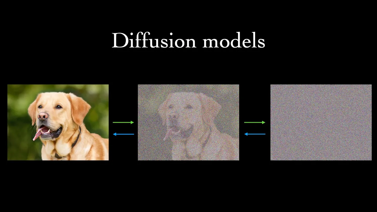
Well it basically starts with random noise and each step it tries to make it slightly less noisy and slightly more like the thing we want. And so going down here is showing all the steps to create the first four, for example, or here to create the first one. And if you look closely, you can kind of see, in this noise, there is something that looks a bit like a one and so it kind of decides to focus on that. And so that's how these diffusion models, basically, work.
So remember, if you're having any trouble finding the materials we're looking at to, go to course.fast.ai or go to the forum topic to see all the links. And this one is called diffusion dash nbs, and the notebook is called —you can see it at the top— stable_diffusion.
Now, a question might be, well why don't we just do it in one go, and we can do it in one go but if we try to do it in one go it doesn't do a very good job. These models aren't, as I speak now in October 2022, smart enough to do it in one go. Now as I mentioned, at the start, the fact that I'm doing it in 51 steps here is, you know, hopelessly out of date because as of yesterday, apparently, we can now do it in three to four steps —I'm not sure if that code's available yet— so by the time you see this, yeah, this might all be dramatically faster, but as I'll be describing, understanding this basic concept —I'm pretty confident it's going to be very important, like, forever— so we'll talk about that. So if we do 16 steps instead of 51 steps, you know, it looks a bit more like it but it's still not amazing.
Okay, so, that's how you can kind of get started and I'll show you a few things that you can tune and, you know, I should remind you that, you know, we're not… most of the stuff I'm showing you in this was built by Pedro Cuenca and the other folks at Hugging Face so, huge thanks to them, there's no way I could have been as up to up to speed with all this detail without their help. They built this library Diffusers and have done a fantastic job of helping display what you can do with it. So let's look at an example of what you can do with it, we're just going to quickly define a little function here to create a grid of images —the details don't matter.
But what we do want to show here is: you can take your prompt, which is “an astronaut riding a horse” and just create four copies of it. Okay so, times, when applied to a list, simply copies the list that many times, so here's a list of the exact same prompt, four times.
And then what we're going to do is we're going to pass to the pipeline the prompts and we're going to use a different parameter now, called “guidance scale”. We're going to be learning about “guidance scale”, in detail, later in the course but basically, what this does is, it says to what degree should we be, kind of, focusing on the specifics caption versus just creating an image. So we're going to try a few different guidance scales, about 1, 3, 7, 14. Generally seven and a half, I believe, at this stage is the default, that may have changed by the time you watch this. And so each row here is a different “guidance scale”.
So you can see, in the first row, it hasn't really listened to us very much at all, these are very weird looking things in there, none of them really look like “astronauts riding a horse”.
At guided scale of 3, they look more like things riding horses, that they might be astronautish and at 7.5 they're certainly, on the whole, look like astronauts riding a horse and at 14 or 15 they certainly look like that but they're getting a little bit too abstract sometimes. I have a pretty strong feeling there are some slight problems with actually how this is coded, or actually how the algorithm works which I will be looking at during this course so maybe, by the time you see this, some of these will be looking a bit better.
I think basically something that's happening here is it's actually, kind of, over… over jumping a bit too far during these high ones.
Anyway, so, the basic idea of what it's doing here is, this guidance is, it's basically actually, for every single prompt, it's creating, creating two versions: one version of the image with the prompt —“an astronaut riding a horse”— and one version of the image with no prompt. So it's just some random thing, and then it takes the average, basically, of those two things.
And that's how, that's what “guidance scale” does, and you can kind of think of the “guidance scale” as being a bit like a number that's used to weight the average.
There's something very similar you can do, where again, you create, get the model to create two images but, rather than taking the average, you can ask it to effectively subtract one from the other. So, here's something that Pedro did of using the prompt a “Labrador in the style of Vermeer”. And then he said, well, what if we then subtract something which is just the model for the caption blue. And you can pass in this thing “negative prompt” to diffusers and what that will do is it will take the prompt, which in this case is “Labrador in the style of Vermeer”, and create a second image, effectively, which is just responding to the prompt “blue” and effectively subtract one from the other, the details are slightly different to that but that's the basic idea, and that way we get a non-blue “Labrador in the style of Vermeer”. So, yeah, this is the basic kind of idea of how to use negative prompt, and you can play with that, good fun.
Here's something else you can play with, is you don't have to just pass in text, you can actually pass in images. So for this you'll need a different pipeline, you'll need an image to image pipeline. And with the image to image pipeline you can grab a rather sketchy looking sketch [Laughter] and you can then pass to this eye to eye image to image pipeline the initial image to start with. And basically what this is going to do is, rather than starting diffusion process with random noise, it's going to basically start it with a noisy version of this drawing and so then it's going to try to create something that matches this caption, and also, like, follows this kind of guiding starting point.
And so as a result, you get things that look quite a lot better than the original drawing but you can see that the composition is the same and so, using this approach, you can, you know, construct things that match the particular kind of composition you're looking for.
So I think that's quite a nifty approach. And so here this parameter “strength” is saying: to what degree do you want to really create something that looks like this or, to what degree do you want the model to be able to, you know, try out different things, a bit.
Now, here's where thing get interesting and this is the kind of stuff you're not going to be able to do at the moment with just the basic GUI's and stuff but, you can, if you really know what you're doing, what we could do now is we could take these output images and we could say: “oh, this one's nice”, sorry, this one. This one's nice, let's make this the initial image. And now we'll say: Let's do an oil painting of… by Van Gogh. And passing the same thing here, and a strength of 1.
And actually that pretty much worked. And I think that's absolutely fascinating, right? because this is something I haven't seen before —which Pedro put together this week— and it's combining simple python code together. And so you can play with that.
Something else you can do —which this one's actually example came from the folks at Lambda Labs— is, and we won't be going into this in detail right now because this is like, basically, exactly like what we've done a thousand times in fastai, is you can take the models in that pipeline and you can pass it your own images, and your own captions.
And so what happened here is… (oh I hate these things, go away, never mind) Here we are. This one, so, what these folks did —I think this was Justin, if I remember correctly— yeah, so, what Justin at Lambda did was he created a really cool data set by going to grab a Pokémon dataset of images, which had almost a thousand images of Pokémon. And then, this is really neat, he then used an imaging captioning —image captioning— model to automatically generate captions for each of those image, images.
And then he fine-tuned the Stable Diffusion model using those image and caption pairs.
So here's an example of one of the captions in one of the images. And then took that fine-tuned model and passed it prompts like “Girl with a girl with a pearl earring” and “Cute Obama creature” and got back these Totoro, these (Oopsy Daisy!)... And got back these super nifty images that now are reflecting the fine tuning dataset that he used and also responding to these prompts.
Here's another example of something you can do. Fine-tuning can take quite a bit of data and quite a bit of time but you can actually do some special kinds of fine-tuning. One that you can do is called Textual Inversion which is where we actually fine-tune just a single embedding. So, for example, we can create a new embedding where we're trying to make things that look like this.
So what we can do is we can give this concept a name.
So here we're going to call it… Oh, I just lost it now.
Watercolor. There we are. We're going to call it “watercolor-portrait”.
And so that's what the embedding name we're going to use is. And we can then basically add that token to the text model and then we can train the embeddings for this so that they match the example pictures that we've seen. And this is going to be much faster because we're just trading a single token for just, in this case, four pictures. And so when we do, that we can then say, for example, “woman reading in the style of” and then passing that token we just trained, and as you see, we'll get back a kind of novel image which I think is, yeah, pretty, pretty interesting.
Another example, very similar to textual inversion, is something called Dreambooth which, as mentioned here, what it does is it takes an existing token but one that isn't used much like, say, “sks” —nothing, almost nothing has “sks”— and fine-tunes a model to bring that token, as it says here, close to the images we provide, and so what Pedro did here was he grabbed some pictures of me and said “painting of sks —so this case he's fine-tuned this token to be Jeremy Howard photos— in the style of Paul Signak”, and there they are. And so the example I showed earlier of the dwarf Jeremy Howard, that service strmr (Astria - https://www.strmr.com/) is actually using this, Dreambooth. So here's how you can try that yourself.
Okay so, that is part one of this lesson which is the: how to get started playing around with Stable Diffusion. In part two we're going to talk about what's actually going on here from a machine learning point of view. So we'll come back in about seven minutes to talk about that. All right, see you guys in about seven minutes.
Okay, welcome back folks. I just thought I'd share with you one more example, actually of textual inversion training this is my daughter's teddy: Tiny —who as you can see is grossly misnamed.
And Pedro and I tried to, yeah, create a textual inversion version of Tiny and I was trying to get Tiny riding a horse and it's interesting that, when I tried to do that, this top row here —this is actually Pedro's example when he ran it— this is showing the kind of steps as he was training, of trying to use the caption “Tiny riding a horse”. And as you can see it never actually ended up generating Tiny riding a horse, instead it ended up generating a horse that looks a little bit like Tiny. And then we're trying to get “Tiny sitting on a pink rug” and actually, after a while it did make some progress there, it doesn't quite look like Tiny. One thing Pedro did that was different to me was he started with the embedding of a person —in my one actually started with the embedding for Teddy and it worked a bit better. But, as you see, there are like problems and we'll understand where those problems come from as we talk more about how this is trained in the rest of this lesson.
Okay so I'm going to be relying on some understanding of the basic idea of how machine learning models are trained here so, if you start getting a bit lost at any point you might want to go back to Part 1 and then come back to this once you're unlost.
The way we're going to start… okay so I need to explain, the way Stable Diffusion is normally explained is focused very much on a particular mathematical derivation.
We've been developing a totally new way of thinking about Stable Diffusion and I'm going to be teaching you that. It's mathematically equivalent to the approach which you'll see in other places but what you'll realize and discover is that it's actually, conceptually much simpler. And also later in this course we'll be showing you some really innovative directions that this can take you when you think of it in this brand new way. So, all of which is to say, when you listen to this, and then you go and look at some blog post and it looks like I'm saying something different, just keep that in mind. I'm not saying something different, I'm expressing it in a different way but it's, it's equally mathematically valid.
What I'm going to do is I'm going to start by saying: let's imagine that… let's imagine that we were trying to get something to generate something much simpler which is to generate handwritten digits, okay. So it's like the Stable Diffusion for handwritten digits.
And we're going to start by assuming there's some like API, some web service or whatever out there —who knows how it was made?— but what it does is something pretty nifty which is that you can get an image of a handwritten digit and you can pass it over into this… this web API into this, you know, this REST endpoint or whatever, it's just a black box as far as we're concerned, and it's going to spit out the probability that, this thing you passed in, is a handwritten digit.
So for this one so, let's say this image is called X1, the probability that X1 is a handwritten digit, it might say is, 0.98.
And so then you pass something else into this magic API endpoint, which looks like this.
You pass that in. And that looks a little bit like an eight, I guess, but it might not be, you'd pass it into this API and see what happens. This is X2 and it says the probability that X2 is a digit is 0.4.
Okay, now we pass in our image X3… into our magic API and it returns the probability that X3 is a handwritten digit… pretty small.
Okay so, why is this interesting. Well, it turns out that if you have a function, you know, let's not call this an API, let's call this, let's call this, it's called “f”, it's some function, but it's like behind some web API REST endpoint, whatever. If you have this function we can actually use it to generate handwritten digits.
So that's something pretty magical and we're going to see how on earth would you do that. If you have this function which can take an image and tell you the probability that that is a handwritten digit, how could you use it to generate new images? Well, imagine you wanted to turn this mess into something that did look like an image. Here's something you could do: let's say it's a 28 by 28 image which is, what? 786… Oopsy Daisy, 28 times 28: 784.
So 784 pixels and we could pick one of these pixels and say: what if I increase this pixel to be a little bit darker? And then we could pass that image through “f” and we could see what happens to the probability that it's a handwritten digit.
So, for a specific example, handwritten digits don't normally have any pixels that are black in the very bottom corners so, if we took this here, and we said: what would happen if we made this a little bit lighter? Right? And then we pass that exact image through here. The probability would probably go up a tiny bit.
For example. So now, we've got an image which is slightly more like a handwritten digit than before and, also, in digits generally, there are straight lines, so this pixel here, it probably makes sense for it to be darker. So if we made a slightly darker version of this pixel, and sent it through here, that would also increase the probability a little bit.
And so we could do that for every single pixel of the 28 by 28, one at a time, finding out which ones: if we make them a little bit lighter, make it more like a handwritten digit, which ones: if we make it a little bit darker, make it more like a handwritten digit.
What we've just done is we've calculated the gradient of the probability that X3 is a handwritten digit with respect to the pixels of X3.
Now, notice that I didn't say “dp(X3) / dX3” —which you might be familiar with from, from high school— and the reason for that is that we've done, we've calculated this for every single pixel. And so, when you do it for lots of different inputs, you have to turn the “d” into a —this is called a del or a nabla— and it just means there's lots of values here. So this here contains lots of values which is the: how much does the probability that X3 is a digit increase as we increase this pixel value, and as we increase this pixel value, as we increase this pixel value. So there's going to be, for 28 by 28 inputs, there's going to be 784 pixels which means that this thing here has 784 values.
Okay, so, with those 784 values they tell us how can we change X3 to make it look more like a digit and so, what we can then do is we can now change the pixels according to this gradient.
And so we can do something a lot like what we do when we train Neural Networks, except instead of changing the weights in a model we're changing the inputs to the model. And so we're going to take every pixel and we're going to modify it: subtract its gradient —a little bit times its gradient— so I multiply this by some constant, let's call it C, and then we're going to subtract it to get some new image. So with the new image, it's probably going to get rid of some of these bits at the bottom, right? And it's probably going to add a few more bits between some of these here, right?
And we've now got something that looks slightly more like a handwritten digit than before.
And this is the basic idea, we can now do that again, we can now take this we can run it through “f” and so we've now got something like, say we call it X3’, for example, so this new version X3’ or whatever it's now the probability that's a handwritten digit —it's quite a bit higher— I'd say it's probably like 0.2, maybe. And we can now do the same thing, we can say for every pixel, if I increase its value a little bit, or decrease its value a little bit, how does it change the probability that this new X3 —whatever prime prime— is a digit. And so we'll now get a new gradient, here, 784 values, and we can use that to change every pixel to make it look a little bit more like a handwritten digit.
So, as you can see, if we have this magic function, we can use it to turn any arbitrary noisy input into something that looks like a valid input, something that has a high P value from that function, by using this derivative. So a key thing to remember here is this saying… is saying: as I change the input pixels, how does it change the probability that this is a digit? And that tells me which pixels to make darker and which pixels to make lighter.
Now, those of you who remember your high school calculus, may recall that when you do this by changing each pixel one at a time to calculate a derivative, this is called the finite differencing method of calculating derivatives, and it's very slow because we have to call —find out diff, uh, sorry— I can't spell diff-e-ren-cing… It's very slow because we have to call it seven of this function, 784 times every single one. We don't have to use finite differencing.
Assuming the folks running this magic API endpoint used Python, we can just call f.backward().
And then we can get X3.grad(), and that will tell us the same thing in one go, by using the analytic derivatives. So we'll learn exactly about what these dot backward does, we'll write our own everything from scratch including our own calculus things from scratch, later, but for now, just like we did in Part 1 of the course, we're just going to assume these things exist.
So maybe then the nice folks that provide this endpoint could actually provide a new endpoint that calls dot backward for us, and gives us dot grad, right? And then we don't really have to use “f” at all, right? We can instead just directly call this endpoint or just directly call this endpoint that gives us the gradient directly, we'll multiply it by this smaller constant C, we'll subtract it from the pixels, and we'll do it a few times, making the input get larger and larger P values, larger and larger probabilities that this is, actually, a digit. So we don't particularly need this thing at all, we don't particularly need the thing that calculates these probabilities. We only need the thing that tells us how… which pixels we should change to calculate the probabilities.
Okay, so, that's great. The problem is: nobody's provided this for us, so, we're going to have to write it. So how are we going to do that?
Well, no problem, generally speaking, in this course, when there's some magic black box that we want to exist and it doesn't exist we create a Neural Net and we train it.
So we want to train a Neural Net that tells us which pixels to change to make a digit look, well, to make an image look more like a handwritten digit. Okay so here's how we can do that, we could create some training data and use that training data to get the information we want, we could pass in something that looks a lot like a handwritten digit, we could pass something that looks a bit like a handwritten digit, we could pass something in that doesn't look very much like a handwritten digit, and we could pass in something which doesn't really look like a handwritten digit at all. Now, you'll notice it was very easy for me to create these, I created real handwritten digits and then I just chucked random noise on top of it.
It's a little bit awkward for us to come up with an exact score saying: how much is that like a handwritten digit? How much is that like a handwritten digit?, how much is that, and how much is that? It seems a bit arbitrary, so let's not do that. Let's use something which is kind of like the opposite, right? and instead let's say: oh, why don't we predict how much noise I added, right? Because this number seven is actually equal to this number seven plus this noise.
And this number three is actually equal to this number three plus this noise.
And this number six is actually equal to this number six plus this noise.
And that one's got a lot. And of course the very first one is equal to this number nine plus this noise.
So, why don't we generate this data and then rather than trying to come up with some arbitrary number of like how much like a digit is it, let's say the amount of noise tells us how much like a digit it is. So something with no noise is very much like a digit and something with lots of noise isn't much like a digit at all. So let's feed in, let's create a Neural Net, who cares what the architecture is, right? It's just a Neural Net of some kind.
And this is critical to your understanding of this course, at this point, we're going to go beyond the idea of like worrying all the time about architectures and details and we're going to be spending, quite often, we're going to get, I mean, we're going to get to all those details but the important thing to using this stuff well is to think about Neural Nets as being something that has some inputs, some outputs, —Oopsy Daisy.
Some outputs. And some loss function which takes those two and then the derivative is used to update the weights, right? That's really what we care about: those four things. Now the inputs to our model is this.
Okay, that's the inputs to our model. The outputs to our model is a measure of how much noise there is. So maybe we could just say: Oh, well, what's the… these are all basically normally distributed random variables, with a mean of zero, and a variance, in this case, of zero. In this case they're normally distributed random variables with mean of zero and a variance of like 0.1.
This one's normally distributed random variables —pixels, I guess— with a mean of zero and like 0.3. This one's super noisy. There's the mean and variance. So that's the mean for each one and the variance for each one. So, why don't we, as the output, use the variance.
So predict how much noise or better still, why don't we predict the actual noise itself.
So why don't we actually use that. Now we're not just predicting how much noise but we predict the actual noise.
That's our outputs. Now if we do that our loss is going to be very simple, it's going to be: we took the input, we passed it through our Neural Net, we tried to predict what the noise was. And so the prediction of the noise is n hat and the actual noise is n and so we can do something we've done a thousand times, which is we can divide it by the count, squared, and then we can sum all that up and this here is the Mean Squared Error, which we use all the time.
So the Mean Squared Error means that we've now got inputs, which is noisy digits, we've got outputs, which is noise, and so this Neural N etwork is trying to predict this noise. So we're basically jumping straight to the step that we had here —remember this is what we really wanted. We wanted some ability to know how much do we have to change a pixel by, to make it more digit-like. Well, tudum! this number seven into this number seven —that's our goal— we have to remove all of that. So if we can predict the noise, then we've got exactly what we want, which is this: we can then do this process, we can take multiply it by a constant and subtract it from our input, and so, if you subtract this noise from this input you get this handwritten digit. So we're doing exactly what we wanted.
Well that seems easy enough, we already know from Part 1 how to do this. So we just have any old Neural Network, so some ConvNeXt, or something that takes as input numbers where we've just randomly added different amounts of noise, lots of noise to some, not much noise to others, it predicts what the noise was that we added, we take the loss between the input, sorry, between… we take the loss between the predicted output and the actual noise, Mean Squared Error, and we use that to update the weights. And so if we train this for a while, then if we pass this into our model, it will return that. And we're done, we now have something that can generate images. How? because now we can take this trained Neural Network —so I'm going to copy it down here— and we can pass it something very, very, very noisy —which is pure noise.
We pass it to the Neural Net and it's going to spit out information saying which part of that does it think is noise, and it's going to leave behind the bits that look the most like a digit, just like we did back here. So it might say: oh!, you know what? if you left behind just that bit, that bit, that bit, that bit, that bit, that bit, that bit, and that bit, it's going to look a little bit more like a digit and then maybe you could increase the values of that bit, that bit, that bit, that bit, that bit and that bit.
And so after you do that —and so that everything else is noise, so we subtract those bits, subtract it times some constant, we're now going to have something that looks more like a digit, which is what we hoped for. And so then we can just do it again. And you can see now why we… you can see now why we are doing this multiple times.
Somebody on the chat saying they don't see me drawing, oh you can see, thanks Jimmy. Son't know Michelangelo what's happening for you.
Okay.
And to answer your earlier question about how am I drawing, I'm using a Graphics Tablet —which I'm not very expert at because on Windows you can just draw directly on the screen, which is why this is particularly messy—.
All right, in practice, at the moment —this might change by the time you've watched this— we use a particular type of Neural Net for this. The particular kind of Neural Net we use is something that was developed for medical imaging called the U-Net.
If you've done previous versions of the course, you'll have seen this, and don't worry this course we'll see exactly how our U-Net works and we'll build them ourselves from scratch.
And this is the first component of Stable Diffusion, it's the U-Net.
Okay so, there's going to be a few pieces and the details of why they're called these things don't matter too much, just yet, just take my word for it this is their names. And the thing that you do need to know for each thing is, like, what's the input and what's the output.
So the input to the U-Net —or what does it do— the input to the U-Net is a, somewhat noisy, image. And when I say somewhat, it could be not noisy at all or it could be all noise, that's the input. And the output is the noise, such that if we subtract the output from the input we end up with the unnoisy image, or at least, an approximation of it.
So that's the U-Net.
Now, here's the problem —well, here's our problem— we have —oh why do I keep forgetting this— we have 28 times 28, 784, I should write that down. We have in these things 784 pixels.
And that's quite a lot. And it gets worse because in practice we don't want to draw handwritten digits, the thing that we'd be passing in here is beautiful high definition photos or images of, like, great paintings. And at the moment the thing we tend to use for that is a 512 by 512 by 3 Channel, RGB. Nice, big image. 512 by 5 12 by 3.
Red, Green and Blue. These are the pixels. So that is 512 by 512. by 3, 786,432. So we've got 786,432 pixels in here and so this is, I don't know, some beautiful picture, this is my amazing portrait, Van Gogh style in a dainty little hat. There we go. So, this is the beautiful painting, or an image of it, it's… that's a lot of pixels and so, training this model where we put noisy versions of millions of these beautiful images is going to take us an awful long time and, you know, if you're Google, with a huge cloud of TPUs or something, maybe that's okay. But for the rest of us we would like to do this as efficiently as possible.
How could we do this more efficiently? Well, when you think about it, in this beautiful picture I drew, storing the exact pixel value of every single pixel is probably not the most efficient way to store it. You know, what if instead, we said like, oh, you know —let's say this is like green rushes or something—.
It might say like, oh over here is green and everything kind of underneath it's pretty much the same, or, you know, maybe I'm wearing a blue top in this beautiful portrait and it could kind of say like, oh, all the pixels in here are blue. You know, you don't really have to do everyone individually, there are faster, more concise ways of storing what an image is.
We know this is true because, for example, a JPEG picture is far fewer bytes than the number of bytes you would get if you multiply its height by its width by its channels.
So we know that it's possible to compress pictures.
So let me show you a really interesting way to compress pictures. Let's take this image and let's put it through a convolutional layer of stride two. Now, if we put it through a convolutional layer of stride two, with six features, with six channels, we would get back a 256 by 256 —gosh that was a terrible attempt at drawing a square, wasn't it?— 256 by 256 —actually do it here— by, okay let's double the number of channels to six, by six. And then let's put it through another stride 2 convolution —and remember we're going to be seeing exactly how to do all these things and building them all from scratch, so don't worry if you're not sure what a stride two convolution exactly is— and just do it again to get 128 by 128, and again, let's double the number of channels. And then let's do it again, another stride two convolutions. So we're just building a Neural Network here.
So now we're down to 64 by 64 by 24, okay, and then now let's put that through a few, like, Resnet blocks, to kind of squish down the number of channels as much as we can, so it'll be now down to, let's say, 64 by 64 by four.
Okay, so here's a Neural Network.
And so the number of pixels in this version is now 64 times 64 times 4, 16,384.
So there's 16,384 pixels here. Okay so, we've compressed it from 786,432 to 16,384, which is a 48 times decrease.
Now that's no use if we've lost our image so, can we get the image back again?
Sure, why not? What if we now create, a kind of, an inverse convolution which does the exact opposite. So, actually let's put it over here. So we're going to take our 64 by 64 by 4 image, put it through an inverse convolution.
So let's put it, let's keep moving this over further back to 128 by 128 by 12. And put it through another inverse convolution, so these are all, just basically, they're just Neural Network layers. 256 by 256 by 6.
And then finally —wrap you out— all the way back to 512 by 512 by 3. Okay, we could put this whole thing inside a Neural Net, here's our single Neural Network.
And what we could do is we can start feeding in images.
It goes all the way through this Neural Network and out at the other end comes back, well, initially it's random, so initially comes out of this is random noise.
512 by 512 well, because I draw it inside here so inside here initially it's going to give us random noise. And so now we need a loss function, right? So the loss function we can create could be, to say, let's take this output and this input and compare them and create and do an MSE, Mean Squared Error directly on those two pieces. So what would that do if we train this model?
This model is going to try to put an image through and going to try to make it so that what comes out the other end is the exact same thing that went into it.
That's what it's going to try to do, because if it does that successfully then the Mean Squared Error would be zero.
So I see some people in the chat saying that this is a U-Net, this is not a U-Net, okay? We'll get to that later, there's no cross connections. It's just a bunch of convolutions that decrease in size, followed by a bunch of convolutions that increase in size.
And so we're going to try to train this model to spit out exactly what it received in.
And that seems really boring, what's the point of a model that only learns to give you back exactly what came in? Well, this is actually extremely interesting. This kind of model is called an auto encoder. It's something that gives you back what you gave it.
And the reason an auto encoder is interesting is because we can split it in half.
Let's grab just this bit.
Okay, let's cut it up, let's grab that just that bit, and then we'll cut a second half —okay they're not quite halves, but you know what I mean— which is just this bit. And so let's say I take this image and I put it through just this first half, this green half which is called the encoder. Okay, I can take this, this thing that comes out of it and I could save it and the thing that I'm going to save is going to be 16,384 bytes.
I started with something that was 48 times bigger than that (786,432 bytes) and I've turned it into something that's 16,384 bytes. I could now attach that to an email, say, or whatever, and I've now got something that's 48 times smaller than my original picture.
So what's going to happen the person who receives these 16,384 bytes. Well, as long as they have a copy of the decoder, on their computer, they can feed those bytes into the decoder and get back the original image. So what we've just done is we've created a compression algorithm.
That's pretty amazing, isn't it? And in fact these compression algorithms work extremely extremely well. And notice that we didn't train this on just this one image, we've trained it on, say, millions and millions of images, right? And then so, you and I both need to have a copy of these two Neural Nets, right? But now we can share thousands of pictures that we send each other by sending just the 16,384 byte version. So we've created a very powerful compression algorithm.
And so maybe you can see where this is going. If this here is something which contains all of the interesting and useful information of the image in 16,384 bytes, why on earth would we train our U-Net with 786,432 pixels of information.
And the answer is: we wouldn't. That would be stupid. Instead we're going to do this entire thing using our encoded version of each picture. So if we want to train this U-Net on 10 million pictures, we put all 10 million pictures through the auto encoder’s encoder, so we've now got 10 million of these smaller things. And then we feed it into the U-Net training hundreds or thousands of times to train our U-Net. And so what will that U-Net now do?
Something slightly different to what we described, it does not anymore take a somewhat noisy image, instead it takes a somewhat noisy -one of these-. So it'd probably help to give this thing a name, and so the name we give this thing is “Latents”. These are called the Latents. Okay, so instead, the input is somewhat noisy Latents. The output is still the noise and so we can now subtract the noise from the slightly noise somewhat noisy Latents and that would give us the actual Latents.
And so we can then take the output of the U-Net and pass it into our auto encoder’s decoder, sorry, uh yes: decoder, because that's something which, okay, that's something which takes Latents and turns it into a picture. So the input to this is small Latents tensor and the output is a large image.
Okay. Now. This thing here is not going to be called an encoder, it's going to have the name the VAE, and we'll learn about why later, those details aren’t too important, but let's put its correct name here the VAE's decoder.
So you're only going to need the encoder for the VAE if you're training a U-Net. If you want to just do inference, like we did today, you're only going to need the decoder of the U-Net.
So this whole thing of Latents is entirely optional, right? This thing we described before works fine. But, you know, generally speaking we would rather not use more compute than necessary so, unless you're trying to sell the world a room full of TPUs, you would probably rather, everybody was doing stuff on the thing that's 48 times smaller.
So the VAE is optional but it saves us a whole lot of time and a whole lot of money. So that's good.
Okay, what's next? Well there's something else which is we have not just been in this morning's, you know, it's in… sorry in the first half of today's lesson we weren't just saying: produce me an image, we were saying: produce me an image of Tiny the teddy bear riding a horse.
So how does that bit work. So the way that bit works is actually, on the whole, pretty straightforward. Let's think about how we could do exactly that for our MNIST example.
How could we get this, so that, rather than just feeding in noise and getting back some digit; how do we get it to give us a particular digit. What if we wanted to pass in the literal number “3” plus some noise and have it attempt to generate a handwritten three for us.
How would we do that? Well, what we could do is, way back here, for the input to this model, why don't is, in addition to passing in the noisy input, let's also pass in a one-hot encoded version of what digit it is.
So we're now passing two things into this model. So previously, this Neural Net took his inputs: just the pixels, but now it's going to take in the pixels and what digit is it as, like, a one-hot encoded vector.
So now it's going to learn how to predict what is the noise, right? And it's going to predict what is the noise and it's going to have some extra information, which is, it's got a know what the original image was so we would expect this model to be better at predicting noise than the previous one because we're giving it more information.
This was a 3, this was a 6, this was a 7. So this Neural Net is going to learn to estimate noise better by taking advantage of the fact that it knows what actual the input was.
And why is that useful? Well the reason that's useful is because now, when we feed in the number 3, like the actual digit 3 as a one hot-encoded vector plus noise, after this has been trained, then our model is going to say: the noise is everything that doesn't represent the number 3, because that's what it's learned to do, right? So that's a pretty straightforward way to give it —and the word we use is: guidance— about what it is that we're actually trying to remove the noise from. And so then we can use that guidance to guide it as to what image we're trying to create.
So that's the basic idea. Now, the problem is, if we want to create a picture of a cute teddy bear, we've got a problem. It was easy enough to pass the digit 8, the literal the literal number eight into our Neural Net because we can just create a one-hot encoded vector in which position number eight is a one and everything else is a zero, but how do we do that for a cute teddy?
We can't. We can't create every possible sentence that can be uttered in the whole world and then create a one hot-encoded version, one-hot encoded version of every sentence in the world because that's going to take a vector that is too long, to say the least.
So we have to do something else to turn this into an embedding, something other than grabbing a one-hot encoded version of this, so what do we do?
So, what we do.
So what we're going to do is we're going to try to create a model that can take a sentence like a cute teddy and can return a vector of numbers that in some way represents what cute teddies look like.
And the way we're going to do that is we're first going to surf the Internet and download images, so here are four examples of images that I found on the internet, and so for each of these images they had an image tag next to them, right?
And if people are being good then they also added an ALT tag to help with accessibility and maybe for SEO purposes and they probably said things like “a graceful swan”.
And the ALT tag for this might have been “a scene from Hitchcock's the birds”.
And the ALT tag for about this might have been “Jeremy Howard”.
And the alt tag for this might have been “fast.ai's logo”.
And we could do that for millions and millions and millions of images that we find on the internet.
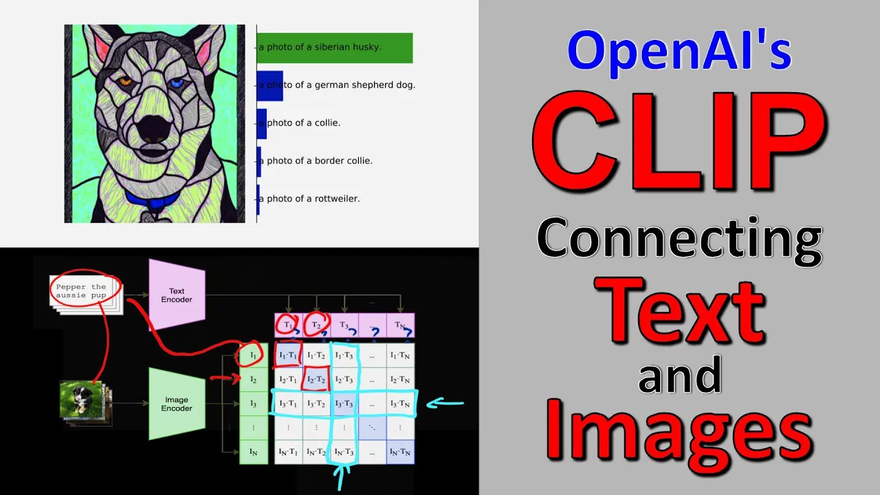
So what we can now do with these is we can create two models. One model, which is a text encoder, and one model, which is an image encoder.
Okay. So again, these are Neural Nets, we don't care about what their architectures are or whatever. We know that they're just black boxes which contain weights, which means they need inputs and outputs and a loss function and then they'll do something.
Once we've defined inputs and outputs and a loss function, the Neural Nets will then do something.
So here's a really interesting idea.
What if we take this image, and what if we then also take the text “a graceful swan”.
Okay, and we're going to feed these into their respective models, which initially they, of course, have random weights and that means that they're going to spit out random features: a vector of stuff, random crap. Because we haven't trained them yet, okay?
And we can do the same thing with a scene from Hitchcock, we pass the scene from Hitchcock in and we'll pass in the words “scene from Hitchcock” and then we'll give us two other vectors, right? And so we can do something really interesting now.
We can line these up —I guess we'll just move them—. We can line these up.
Okay, here's all of our images, okay? And then we can have —Oopsy Daisy—.
Okay, and then we can have our text.
So we've got “graceful swan”, we've got “Hitchcock”, we've got “Jeremy Howard”, and we've got fastai logo.
Now, ideally, when we pass the “graceful swan” through our model, what we'd like is that it creates a set of embeddings that are a good match for the text “graceful swan”.
When we pass the scene from Hitchcock through our image model we would like it to return embeddings which are similar to the embeddings for the text seen from “Hitchcock” and ditto for the picture of Jeremy Howard versus the name “Jeremy Howard” and ditto for the image fastai and (sorry). The fastai logo and the word “fastai logo”. So, in other words, for this particular combination here, we would like this one's features and this one's features to be similar.
So, how do we tell if two sets of things are similar? Two vectors?
Well, what we can do is we can simply multiply them together, element wise, and add them up.
And this thing here is called the dot product.
And so we could take the dot product of the features from the image model for this one and the dot product of the features from the text model for the word “graceful swan” and take that dot product. And we want that number to be nice and big.
And the scene from Hitchcock's features should be very similar to the text scene from Hitchcock's features, so we want their product to be nice and big. And ditto for everything on this diagonal.
Now, on the other hand a graceful swan picture should not have embeddings that are similar to the text “a seen from Hitchcock”.
So that should be nice and small. And ditto for everything else off diagonal.
And so perhaps you can see where this is going. If we add up all of these, right? Add those all together and then subtract all of these: we have a loss function.
And so, if we want this loss function to be good, then we're going to need the weights of our model, for the text encoder, to spit out embeddings that are very similar to the images that they're paired with. And we need them to spit out embed… features, for things that they are not paired with, which are not similar.
And so if we can do that then, we're going to end up with a text encoder that we can feed in things like “a graceful swan”, “some beautiful swan”, “such a lovely swan”, and these should all give very similar embeddings, because these would all represent very similar pictures. And so what we've now done is we've successfully created two models, that together, put text and images into the same space. So we've got this multimodal set of models, which is exactly what we wanted. So now, we can take our cute teddy bear, feed it in here, get out some features and that is what we will use instead of these one-hot encoded vectors when we train our photo, or painting, whatever U-Net. And then we can do exactly the same thing with guidance, we can now pass in the text encoder’s feature vector for a cute teddy, and it is going to turn the noise into something that is similar to things that it's previously seen that are cute teddies.
So the model that's used, or the pair of models that's used here, is called CLIP.
This thing where we want these to be bigger and these to be smaller is called a contrastive loss.
And now you know where the CL comes from. So here we have a CLIP text encoder.
Its input is some text. Its output is, we call it an embedding, it's just some features.
Oops, embedding, where similar sets of text, meaning, with similar meanings, will give us similar embeddings.
Okay —because we need a bit more space— we're nearly done.
Okay, so we've got the U-Net that can denoise latents into unnoisy latents, including pure noise. We've got a decoder that can take latents and create an image.
We've got a text encoder which can allow us to train a U-Net which is guided by captions.
So the last thing we need is the question about: how exactly do we do this inference process here?
So, how exactly, once we've got something that gives us the gradients we want… and by the way, these gradients are often called the “score function”, just in case you come across that, that's all that's referring to. Yeah, how exactly do we go about this process?
And, unfortunately, the language used around this is weird and confusing and so, ideally, you will learn to ignore the fact that the language is weird and confusing. And in particular the language you'll see a lot talks about “time steps”.
And you'll notice that during our training process we never used any concept of “time steps”. This is basically an overhang from the particular way in which the math was formulated in the first papers.
There are lots of other ways we can formulate it and during the course, on the whole, we will avoid using the term “time steps”. But we can, to see what time steps are, even though it's got nothing to do with time in real life, consider the fact that we used varying levels of noise, some things were very noisy, some things were not noisy at all, some things had no noise and some I haven't drawn here would have been pure noise.
You could basically create a kind of a noising schedule.
Where along here, you could put, say, the numbers from 1 to a 1,000, and you could then say: oh, you know —and we'll call this “t”— and maybe we've randomly pick a number from 1 to a 1,000, and then we look up on this noise schedule —there should be some monotonically decreasing function— and we'd look up, let's say we happen to pick randomly, a number 4, we would look up here to find where that is and we'd look over here and this would return to us some Sigma, which is the amount of noise to use if you happen to get a 4.
So if you happen to get a 1 you're going to get a whole lot of noise, and if you happen to get a 1,000 you're going to have hardly any noise.
So this is one way of, like, picking… so remember we were going to pick in, when we were training, we were going to pick for every image a random amount of noise. So this would be one way to do that, is to pick a random number from 1 to a 1,000, look it up on this function and that tells us how much noise to use. So this “t” is what people refer to as the time step.
Nowadays you don't really have to do that that much and a lot of people are starting to get rid of this idea altogether and some people instead will simply say how much noise was there. Normally we would think of using Sigma for standard deviations of gaussians or normal distributions, but actually, much more common is to use the Greek letter Beta. And so if you see something talking about Beta, they're just saying: oh, for that particular image, when it was being trained, what standard deviation of noise was being used, basically. Slightly hand wavy but close enough.
And so what you do, each time you're going to create a mini batch to pass into your model, you randomly pick an image from your training set you, randomly pick either an amount of noise or, since some models you randomly pick a “t” and then look up an amount of noise and then you put use that amount of noise to each one and then you pass that mini batch into your model to train it. And that trains the weights in your model so it can learn to predict noise. And so then, when you come to inference time —so inference is when you're generating a picture from pure noise— you want your model, you're basically, your model is now starting here, right? Which is as much noise as possible. And so you want it to learn to remove noise, but what it does in practice, as we saw in our notebook, is, it actually creates some hideous and rather random kind of thing.
So in fact let's remind ourselves what that looked like.
This is what I created, when we tried to do it in one step. So remember, what we then do is we say: okay, what's the prediction of the noise and then we multiply the prediction of the noise, I said, by some constant —which is kind of like a learning rate— but we're not updating weights now, we're updating pixels. And we subtract it from the pixels.
So, it didn't actually predict the image, what it actually did was it predicted what the noise is, so that could then subtract that from the image, from the noisy image, to give us the denoised image. And so, what we do is we don't actually subtract all of it, we multiply that by a constant and we get a somewhat noisy image.
The reason we don't jump all the way to the best image we can find is because things that look like this never appeared in our training set and so, since it never appeared in our training set, our model has no idea what to do with it. Our model only knows how to deal with things that look like, somewhat noisy latents, and so that's why we subtract just a bit of the noise so that we still have a somewhat noisy latent.
So, this process repeats a bunch of times and questions like: what do we use for C?
Right? And, how do we go from the prediction of noise to the thing that we subtract? These are all of the things that are the the kind of the things that you decide in the actual sampler.
And that's used both to think about, like, how do I add the noise? and how do I subtract the noise?
And there's a few things that might be jumping into your head at this point, if you're anything like me, and one is that, gosh, this looks an awful lot like Deep Learning optimizers.
So in a Deep Learning optimizer this constant is called the Learning Rate. And we have some neat tricks where we say, for example, oh, if you change the same parameters by a similar amount, multiple times in multiple steps, maybe you should increase the amount you change them, this concept is something we call Momentum.
And we'll be doing all this from scratch during the course, don't worry, and in fact we even got better ways of doing that, where we kind of say, well, what about what happens if the variance changes, maybe we can look at that as well and that gives us something called Adam. And these are types of optimizer.
And so maybe you might be wondering: could we use these kinds of tricks?
And the answer, based on our very early research is yes, yes we can.
The whole world of, like, where Stable Diffusion and all these diffusion-based models came from, came from a very different world of maths, which is the world of differential equations.
And there's a whole lot of very parallel concepts in the world of differential equations, which is really all about taking these like little steps, little steps, little steps and trying to figure out how to take bigger steps. And so, different differential equation solvers use a lot of the same kind of ideas, if you squint, as optimizers.
One thing the differential equations solvers do, which is kind of interesting though, is that they tend to take “t” as an input. And in fact, pretty much all diffusion models —I've actually lied—, pretty much all diffusion models, don't just take the input pixels and the digit, or the caption, or the prompt they also take “t”. And the idea is that the model will be better at removing the noise if you tell it how much noise there is. And remember, this is related to how much noise there is.
I very strongly suspect that this premise is incorrect, because if you think about it. for a complicated fancy Neural Net figuring out how noisy something is, is very, very straightforward.
So I very much doubt we actually need to pass in “t”. And as soon as you stop doing that, things stop looking like differential equations and they start looking more like optimizers. And so, actually, Johno started playing with this and experimenting a bit and early results suggest that, yeah, actually when we re-think about the whole thing as being about learning rates and optimizers, maybe it actually works a bit better. In fact there's all kinds of things we could do. Once we stop thinking about them as differential equations and worry about the math —don't worry about the math so much about gaussians and whatever— we can really switch things around. So for example, we decided, for no particular obvious reason, to use MSC. Well, the truth is, in statistics and Machine Learning almost every time you see somebody use MSE it's because the math worked out better that way. Not as in: it's a better thing to do but, as in, you know, it was kind of easier.
Now, MSE does fall out quite nicely as being a good thing to do with some particular premises, you know, like it's not like totally arbitrary but, what if we instead used more sophisticated loss functions where we actually said, well, you know, after we subtract the outputs, how good is this really? Does it look like a digit? or, does it have the similar qualities to a digit?
So, we'll learn about this stuff, but this thing is called, for example, Perceptual Loss.
Or another question is, do we really need to do this thing where we actually put noise back at all?, could we instead use this directly?
These are all things that suddenly become possible when we start thinking of this as an optimization problem rather than a differential equation solving problem. So, for those of you are interested in, kind of, doing novel research, this is some of the kind of stuff that we are starting to research at the moment and the early results are extremely positive, both in terms of how quickly we can do things and what kind of outputs we seem to be getting.
Okay, so, I think that's probably a good place to stop it. So what we're going to do in the next lesson is we're going to finish our journey into this notebook to see some of the code behind the scenes of what's in a pipeline when I get there.
So we'll be looking inside the pipeline and see exactly what's going on behind the scenes a bit more in terms of the code. And then we're going to do a huge rewind to the “from the foundations” and we're going to build up from some very tricky ground drills. Our ground drills would be we're only allowed to use pure Python, the Python standard library and nothing else, and build up from there until we have recreated all of this, and possibly, some new research directions at the same time.
So that's our goal and so strap in and see you all next time. See ya!
Up Next
43:18
Implementing Stable Diffusion VAE in PyTorch: A Step-by-Step Guide (50 chars)
@freecodecamp
31.1K views•2024-12-04

57:48
Secure Multiparty Computation (MPC): Foundations & Challenges
@SimonsInstitute
7.3K views•2015-05-28

91:13
Language Models Guide: Fast.ai's Jeremy Howard on GPT-4 and Fine-Tuning
@howardjeremyp
567.9K views•2023-09-24

18:41
Neural Networks Explained: Math, Layers, and Learning Fundamentals
@3blue1brown
21.9M views•2017-10-05
Related Study Plans & Knowledge Roadmaps
Structured learning paths in Artificial Intelligence
artificial-intelligence
Aligning LLMs: DPO, TRL & Custom Datasets
01Foundations of Python & Machine Learning
02Transformers and Large Language Models (LLMs)
03Aligning LLMs: SFT and RLHF
+ 3 more learning modules
24h6 modules
Explore Roadmap
artificial-intelligence
Federated Learning: PyTorch, Flower & Privacy
01Python & Machine Learning Foundations
02Deep Learning Basics with PyTorch
03Introduction to Federated Learning
+ 2 more learning modules
35h5 modules
Explore Roadmap
artificial-intelligence
Securing LLMs: Guardrails AI & NeMo Gateway
01Introduction to LLMs, Python, and APIs
02Understanding LLM Vulnerabilities & Threats
03Defending LLMs with Guardrails AI
+ 2 more learning modules
15h5 modules
Explore Roadmap
artificial-intelligence
Building Recommenders: Two-Tower & Vector DBs
01Foundations of Python & Machine Learning Basics
02Introduction to Recommender Systems
03Deep Learning & Representation Learning
+ 3 more learning modules
75h6 modules
Explore Roadmap