

















In projective 2D space, conics (parabolas, ellipses, hyperbolas) are represented by homogeneous equations x^T C x = 0 with five degrees of freedom, requiring five points to uniquely define them; degenerate conics occur when the matrix rank drops below 3, representing either a single line (rank 1) or two intersecting lines (rank 2). Projective transformations (homographies) are invertible 3×3 matrices preserving collinearity, forming a hierarchy from Euclidean transformations (preserving distance and angles) through similarity transformations (preserving shape) to affine transformations (preserving parallelism), with the most general projective transformation having eight degrees of freedom and being computable from four point correspondences.
3D Computer Vision: Lecture 1 Part 2 - Projective Geometry
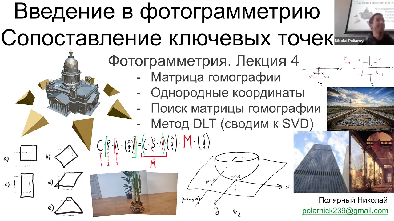
Added:so after looking at the homogeneous representation of points and lines we'll now look at the representation of konigs in the projective 2d space a coding is actually a curve described by a second degree polynomial equation in the plane on the cartesian coordinates and in euclidean geometry conics are of three main types namely the hyperbola the ellipse as well as the parabola and we'll see in the next slide that how this three different types of conics are generated from geometry and these three types of conics arises as conic sections generated by planes differing from or of differing orientation we'll see in the next slide that this is in fact the intersection of planes of different orientation that intersects two inverted cones and note that besides these three different types of conics there are also degenerate conics which we will define later so here's the illustration of how the three main types of conics arises from geometry the first type which is parabola it occurs when a plane intersects the two inverted conics uh at the location or at an orientation such that the tangent to this plane is aligned with the axis with the side axis or tilted axis of the two inverted conics over here so in this case here the intersection of the plane with the two inverted conics which is given by this curve over here would define a parabola conic and in the case where the tangent of the plane is aligned with the base of the or parallel with a base of the inverted cones then this will give rise the intersection will give rise to a sucker and if it is tilted at a certain angle but it's still close to the the tangent of the plane is too close to the the alignment with the base of the circle then this will give rise to the ellipse conics and in the case where the tangent of the plane is aligned with the vertical axis parallel with the vertical axis of the inverted cones then the intersection of this plane with the inverted cones would give rise to the hyperbola so now having a look at the geometric intuition behind how the three different types of chronics are formed let's go into the mathematical formulation of konigs so we all know that the equation of conics in inhomogeneous coordinates or cartesian space coordinates is actually a two degree polynomial given by this particular equation here so let us follow the concept behind the homogeneous conversion of a point where we saw that a point x can be represented as homogeneous coordinate of x 1 x 2 and x 3 where we simply replace x with x1 divided by x3 and x2 divided by x3 to get the homogeneous coordinates and or to get the coordinates in the cartesian space so this is a conversion behind between homogeneous coordinates and the cartesian coordinates that we are familiar with and in in this case here we are simply divide we simply divide the homogeneous coordinates the first two elements of the homogeneous coordinates with the third uh coordinate over here and uh we'll do the same here we'll simply uh replace x over here with uh x1 divided by x3 and x and y over here uh to be replaced by x2 divided by x3 to get this particular equation here so uh here we will replace this x and y over here so since this guy here is equivalent to x and y we'll simply use these two equations over here two relation over here to convert from cartesian to homogeneous coordinate so now the homogeneous representation of the equation of conics we can see that it's a parameterized by x1 x2 and x3 with the coefficients of a to f that remains intact here now we can rewrite the homogeneous form of the konigs equation into a metric form which is given by x transpose of c multiplied by x equals to 0 where x here is simply x 1 x x2 and x3 and c here would be in terms of this matrix form over here is a three by three matrix and now we can say that c is a homogeneous representation of a conic and here only the ratio of the matrix elements are important multiplying c by a non-zero scalar has no no effect this is similar to the homogeneous representation of a line and the homogeneous representation of a point we can see that because this is a this equates to zero multiplied by any k scalar value it will always cancel out and hence there's no effect on the konigs equation here the conics can be seen to have five degrees of freedom which is can be thought of as a ratio of a b c d e and f since we said just now that multiplying the konigs equation with a k here would have no effect this means that it's only the ratio of these six values the six parameters of the conics that is important and uh in this case here what we say is that uh it's also equivalently that the six elements of the symmetric metric uh less one for the scale which is given by k over here and hence it's a five degrees of freedom so each point on the conic's x i which we denote as x i the coordinates are x i and y i places one constraint on the conics coefficient given by this second degree polynomial equation over here and what this means geometrically is that given a conic for example this ellipse over here when we have one point that lies on this particular coding this is going to give one of this constraint and this particular constraint in terms of this polynomial equation can be written rewritten in a metric form or in a metric or in a homogeneous linear equation formed as this particular case so this is equivalent to a vector or dot product of vector which will give us a 0 over here where c this vector c here is the coefficients of the conics a b c d and e represented as a six vector here so uh since we have six unknowns inside the uh inside this six factor over here this guy here is a six factor which is actually a six unknowns over here oh what it means here is that two in order to solve for the six unknown where the less one minus one for the scale this means that we have looked at this earlier that there's only five degrees of freedom that defines the conics of the of c over here so what it means is that we only need five constraints we only need a total of five constraints or minima number of uh five constraints to in order for us to solve for the unknown conics so geometrically what this means is that uh in order to solve for these coding we need to know five points on these conics in order to solve for the koenigs equation here which is represented by c and stacking this up together we'll get a homogeneous linear equation where this guy here is equals to a and which is a five by six matrix and c here is actually a six by one vector and this would be equals to zero or what this means in linear algebra is that c here the solution of c here lies in the null space of the matrix of a here and once this five points are known this means that this coefficient here the the matrix of a here would be all known a known value we can easily solve for the null space of a to get the solution of c which represents the konig equation we'll see in the later lecture that this can be easily solved by doing the svd the singular value decomposition of a and to get the null space of a which will be the solution of c here and uh one interesting thing to note here is the tangent lines to the conics this is also uh the intersection the intersection of a line with a konig and this will give rise to a point when this line forms a tangent to the conics we'll also see the later the in the degenerate cases that that sometimes the line might also intersect at two points or sometimes the line will not intersect and but in this case here we'll look at the case where the line actually uh is a tangent line to the conics and when this happens uh this tangent line to the coding is actually intersecting at a point which we denote as x given by this equation over here l equals to c x let's uh here's the proof uh in the algebraic sense so the line uh l equals to cx passes through x this means uh which is denoted as the in this figure over here uh this means that this line is actually a tangent line to the conic c since there's only a unique point of intersection here at x since l x l transpose x equals to x transpose c x equals to 0. so l transpose x is what we have learned earlier the when the point x lies on the line l then this l transpose x or the duality x transpose l is going to be equals to zero so in this case here we are using this l transpose x equals to zero and we have also seen that uh the all the points that lies in the konig is going to fulfill this uh incidence relation where x transpose c x equals to zero so if the line has one contact point which means that this line is actually the tangent line to the conic then it is a tangent and we are done and we can see that uh in this case here the l here and l here that fulfills this since there's only one point of contact which is a tangent line then l here would we can rewrite this l transpose equals to x transpose of c which also implies that l is equals to c of x here hence we have proven that the tangent line intersects the conic at l equals to c x now the chronic that we have defined so far it should be properly termed as a point conic as it is uniquely defined by a equation on points this is because the second degree polynomial that we look at it's defining a point on uh coding and we saw earlier that five of these points that lie on the conic uniquely defines the conic and there is also a dual to the cloning as in the dual of a line so previously in the previous slide we saw that there is a point line duality given by x transpose l equals to l transpose x equals to zero and this duality actually means that uh we can define a line with a point and interchange the point with a line as well so what this means is that uh you can see that if i have many points over here it actually can be used to represent a line and if i have a line here it can be at the same time used to represent this many points on the line so here uh there is also a duality between the line conic and the point conics so a point coding is what we have defined earlier which is uniquely defined by a set of five points or more than five points so anything that is more than or equal to five point can be used to uniquely define this particular conic and we can also do the same with lines so we can see that the chronic can be uniquely defined with tangents of the line so if i have many tangents of the using the line onto a conic i can actually use it to uniquely define my conics and this relation here is given by this equation over here l transpose c star l equals to 0. we define c star over here to be the dual conics which is defined by the line or in other words this is actually just the line coding so we can see that the analogy would be our poinconics which is what the equation that we saw earlier is x transpose c x equals to zero so this means that the x here lies on the uh the the point here lies on the conics and in this case here it means that the lines lies on the conics c star so this case here is a c and we have all the points of x and this case here the dual conics will have all the lines denoted as l and a dual conics also has five degrees of freedom and what this means is that the conics can also be computed from five unique lines that define the conics and for a non-singular symmetric metric c star it's uh the dual conics denoted by c star over here is actually given by the inverse of the uh conics of the poinconics so we can write c star equals to c inverse up to a certain scale so uh the proof is here the let's given a point x on the on the conic c so let's say this is chronic c and given a point x over here that lies on the conic c the tangent is we have seen in the previous slide that the tangent is given by the this equation here l equals to c over x uh c c multiplied by x over here and this implies that in this case if c is invertible x would be equals to c inverse l and this means that we can rewrite this c inverse here with c star which gives us this equation this relation over here uh which is the dual of this l equals to c this tangent line so uh in this case here we will have a point c star this defines c star over here where we have a point that defines uh by the line that is tangent to this c star over here hence this particular relation over here furthermore since x satisfies this equation the second degree polynomial equation that we have seen earlier we obtain this relation by substituting the uh point with this equation this particular relation over here by substituting x with c inverse of l into x over here into two sides of this quadratic equation over here and simplifying this since this is a transpose c inverse l transpose will give us l transpose c inverse transpose over here and uh what we can see here is that we will end up to have this equation over here since since c and c inverse is equals to identity and c inverse transpose is equals to c inverse hence we'll get this particular relation over here and as a result we can see that this relation can be rewritten into l transpose c star l equals to 0 by simply saying that the dual conics is equals to the inverse of the coding and geometrically dual conics are also known as the chronic envelopes because i have said earlier that the uh do lower line conics here is defined by all the tangent lines as compared to the poi chronic as compared to the point conics which are defined by points on the conic so five or more than or equal to five points can uniquely define this conic c and here in the same case here we have more than or equals to five lines uh tangent lines to the conic we can define the line conic c star now suppose that in addition to x there's another point of intersection of the tangent line to the conics which we denote as y over here and uh it follows that then y transpose c y would be equal to 0 following the equation that we have seen of earlier of x transpose c x equals to 0 and we know that since this particular point of y must lie on the line l then the intersection or equation over here the the incidence equation over here l transpose of y must be also equals to zero uh it will hold and we have also seen that there is another point of x earlier that this must be the intersection of the tangent line and the conics therefore the equation l equals to c x must also be true and if we were to replace this particular l equals to c x in this equation over here then we will get another relation of x transpose c y equals to l transpose y equals to 0 over here and interestingly it follows that if all these relations uh holds true that means that for the tangent line there are actually two points that of intersection with the conics then it follows that this relation here must be true for all alpha and what it simply means here is that x plus alpha y is another point on the on the line and uh what happens here is that x plus alpha y it actually means the line itself and uh this simply means that i have two points x and y and any magnitude of this y is going to denote any point on this particular line over here and what this means is that if this if there's another point of y in addition to x that lies on the intersection of the tangent line to the conic then the whole line joining x and y over here the whole line here must lie on the konig so what this means here is that the konig will no longer be ellipse hyperbola or parabola shape or even a circle shape it means that the ellipse now or this conics now must also take a straight line therefore the tangent line to this conic which is also a straight line would have all the points lying on the conic and we say that this kind of conics is a degenerate chronic we will look at several cases of these degenerate conics so we have seen algebraically that the conic degenerates when we say that any line that is uh tangent to the conic intersects the chronic at every single point here in uh that is given by this equation here so what this means is that given a line which is uh spam by x and y these two points over here the conic is degenerate when it meets this particular tangent line at every point of the line that is span by x and y and there are geometrically three cases where this can happen in the first case where x and y actually collapse to a singular point this means that they are actually x is equals to y over here and in this case geometrically what this means is that we will have the plane intersecting at the intersecting point of the peaks of the two cones over here and in this case we can see that this particular conex over here fulfills this equation for whichever x and y and uh in the second case we can see that the uh it happens when the plane intersects exactly at the slanted axis of the inverted cones over here and in this case we can see that this intersection forms the line this particular line over here so this is the cooling c over here and any points we can see very clearly from this uh illustration over here that any points on this line will still lie on this particular conic itself because the cloning itself is a line and in the third case the conics would be intersecting the two inverted cones or the plane will be intersecting the two inverted cones in this manner over here which it forms two straight lines over here and in this case whatever lines or whatever points that lies on either one of these two straight lines would also fulfill this particular equation over here and they will all fulfill these two sets of equations since we are saying that both x and y now of the tangent line that lies on the tangent line as well as it must lie on the conics itself we'll see that in order for this to happen the rank of c must be less than 3. so i have mentioned earlier in the previous slide that if the metric is not full rank then the konig is termed as degenerate what this means is that the rank of c here must be lesser than three because c is actually a three by three square matrix and anything the rank lesser than three this means that the metric is not full rank and the degenerate clinics uh that will include two lines and a repeated line of rank two and rank one we will look at these two cases or after the example so in the first case where we are looking at here is that the codex is consists of two lines and we'll see that it actually forms a rank two konig and in this case this chronic can be formed by uh two lines which i denote as l and m over here and uh taking l multiplied by m transpose this is the dot product and plus the transpose of this dot product we'll see that we'll get the rank two conics over here and uh indeed after putting into the this particular equation over here which is the coordinate equation that we have seen earlier that uh from the two sets of equations over here the the two summation terms over here multiplying it by uh x and x transpose and x over here and we can see that uh this indeed gives us zero and since from this particular equation here which is the chronic equation that we have seen earlier that it actually reviews the two lines where the first term here the dot product of x and l denotes the first line equation of l which is the line and the point that is lying on the line as well as the second term here which is the dot product of m transpose and x over here where m is my second line and x is the point that lies on the line so we can see that from this particular formulation here it actually reviews two line equations over here and hence the degenerate conic in this case where the rank is equal to two it's actually uh two lines which is represented geometrically from this uh using this particular figure over here and in the second case we can see that uh if the rank of the matrix is equals to 1 this means that the rank of the c matrix the chronic matrix equals to 1 then c is actually the conic is actually a repeated line which overlaps each other the same line given by this case over here so l transpose l uh plus l or l transpose is going to give me a repeated line and with the rank of c here equals to 1 and in this case we can put it into the we can put the same equation over here into our konigs equation to get this particular relationship which is equals to zero over here and here it's not difficult to see that uh after putting it into this particular relationship over here we can see that this actually consists of two terms which is the dual of each other which highlights the point line relationship over here and hence l here and the l over here would be the same repeated line with rank of one forming the codings so there also exists degenerate dual conics or dual line conics that includes two points of rank two and a repeated point of rank 1 as we have seen in the first case of the illustrations of the geometric illustrations of the degenerate codings earlier and in this case here an example would be the line conics c star equals to x y transpose plus y x transpose so this is of of rank two which consists of uh which consists of two points over here that is a form in the in this way so though the reason why it has to be formed in this way the because c is actually a symmetrical square matrix so the way that it's formed in this way the it will ensure that c the resulting c is a valid conics and uh it will also ensure that it has a rank two and this dual conics consists of lines passing through either of the two points x or y so what this means is that it will form something like this where i have x and y over here and this point would be made up of all these lines that is intersecting on the point over here and similar formulation can also be done for the rank one line conics of the repeated points so i won't go into the proof or i won't go to show that this is indeed the set of points because as i have mentioned earlier that the duality principle means that as long as i have shown it for the points conics the same relation should also hold for the dual line conics over here and note that in this case here c star which is my dual conic the inverse of this is not equal to c as what we have mentioned earlier that if the rank of c is full rank which is equals to 3 then c star would be equals to c inverse but in this case since the rank of c is not equals to 3 then this relation doesn't hold anymore now after looking at the definitions of points lines and conics in the homogeneous coordinate space and in the 2d projective space let's look at how these entities can be transformed in the 2d projective space so 2d projectives geometry as i mentioned is actually a study of the properties of the projective plane they are invariant under group transformation known as projective so as i have illustrated earlier on that uh in the in this case here the 2d projective geometry is can be seen as the ray forming on projecting onto each one of this plane to form a line or it could be the plane that is intersecting on the uh on this individual planes of k equals to 1 k goes to 2 okay k can actually be any real number here the intersection here to form a line and a conics etc so in this case here when we are starting the 2d projective geometry we are studying uh how this transformation of these planes that intersects the line the plane or the inverted cones can result in the invariance or certain invariant property after the transformation and specifically a projectivity needs to be an invertible mapping which we denote hsh from p2 to p2 itself so this means that i'm mapping any input point or to or input entity in the 2d projective space it could be a point line or conex and the mapping should also be mapped into a projective 2d space denoted by h and this linear mapping simply means that if i have a point i denote this h as a mapping it should be able to rewrite it into this form where it becomes a linear mapping and it should also be invertible this implies that i should be able to recover x prime from the inverse of h multiplied by x over here and this means that the mapping from one space projective space to another would be denoted as h and the inverse of this would bring me back from the other space back to the original space so a projectivity is also called a collineation or a projective transformation or simply a homography the theorem of projective space is that as i mentioned in the previous slide is that given a mapping edge it actually maps an entity from a 2d projective space into a another 2d projective space and this is a projective this mapping is a projectivity if and only if there exists a non-singular 3x3 matrix h here which we denote as capital h over here such that any point in the 2d projective space represented by a vector is true that the mapping follows this particular function over here so in this case i would have mapped it into x prime given by h multiplied by x and both of x and x prime both of x and x prime must be in the 2d projective space and as well as h here must also be an invertible entity where we will skip the full proof so the partial proof begins with let's x1 and x2 and x3 lie on a line so these three are lying on the line x1 x2 and x3 thus this equation of the line point incidence relation goes through where the dot product of the line and the points will be equals to zero for one two and three and let h be a non-singular three by three matrix so we can verify that uh after the mapping after this mapping with h as i have mentioned in the very beginning of the lecture that despite that the geometrical properties of many shapes and geometry structures change when it undergoes a projective transformation the straightness of it will not be changed so what this means is that if i were to map these three points on the using this homography of age then it would be mapped from it would be transformed from a p2 space to another p2 space but in after the transformation these three points should also appear collinear to each other we can easily verify this by doing this so a projective transformation of l is given by this guy over here and a projective transformation of x is given by uh this guy over here so in this case i'm mapping the line independently from the points and we can see that by putting both of them together so this will end up to have l prime which is this guy over here l prime after the mapping l to l prime and this h x i would be my points of x i prime over here and this would be x i over here so putting them together in the coincidence relation i will still get 0 because h inverse and h cancels out what this means is that as a result after the transformation my l prime multiplied by the x i prime over here it will still be equal to zero what this means is that all the three points after the mapping after the homography mapping it will still be collinear to each other and it will still be lying on the line hence the collinearity is preserved by the transformation so what we want h to follow would be this we want to find an h such that it's capable of mapping p2 space to p2 space where the collinearity is preserved and it's a linear mapping which is invertible following the principles or following the rules that we have laid out earlier for the projective transformation h we now define the planar projective transformation in this matrix form let's denote the p2 space the final p2 space as x of x prime over here as x1 prime x2 prime x3 prime over here and h here would be a three by three matrix that it's capable of doing linear projection or linear transformation of my original point x in the p2 space as well and it will map this p2 space into another p2 space of x prime over here or simply we'll write this linear mapping relation as x prime equals to h multiplied by x and here's some properties of h it has to be a non-singular 3x3 matrix because as mentioned before h needs to be able to be inverted and hence it has to be a non-singular matrix for this relation to hold true it also has to be a homogeneous matrix since only the ratio of the matrix of the elements is significant and it has to be 8 degrees of freedom we will see later on why it has to be 8 degrees of freedom among the 9 elements of age when we learn about the robust estimation of homography in the later lecture now geometrically what the transformation what the homography transformation of projective transformation means is that we are actually trying to find a linear mapping such that as we have mentioned that x or any point it's represented by the intersection of the ray with the plane so what we are trying to do here with the linear mapping is that instead of planes that are parallel to each other which we have denoted using our homogeneous coordinates of x y and k or k x k y and k over here we say that by varying this particular ray over here is intersected by all the planes that are parallel to each other at a different interval different k interval so in this case here it represents the same point but a linear mapping homogeneous linear mapping simply means that i want to find after i have transformed this plane into another plane which is not uh paler to this particular plane over here by considering the same line the same ray that intersects these two planes here the relation between these two points which i call x prime and x over here would be related by a homography which can be written as x prime equals to h multiplied by x and hence the projective transformation of x prime equals to h multiplied by x can arise in perspective images the examples some examples will be given here and these are the unique cases where this particular transformation can be valid it doesn't hold in all cases but it has to be a transformation from planes to planes because as what we have defined in the earlier slide is that the what we're interested in would be the the origin with a ray i want to find the intersection of this particular ray with different planes and the relation between these two points here for example which intersects the which is the intersection of the planes of with this particular line over here would be related by the homography equation hence it has to be a point lying on the plane in order for this to be valid and another uh part that it has to be valid would be it has to be a perspective uh images what they mean what this means is that all this light rays all these rays over here it has to converge at the single point of convergence we'll look at this in the future lecture in more detail but here we'll study the properties of this homography on different geometrical structure so we have seen earlier that uh if a point x i lies on a line then the transform point x i prime would be equals to h multiplied by x i under projective transformation and this after the projective transformation this points over here which originally lies on the line so all these points which i denote generally as x i that lies on the line l it would be still lying on a line after the transformation which i denote as l prime over here and this point over here would be x i prime after the homography or the projective transformation and the transformation of the point would be given by x prime equals to h multiplied by x i uh and the projection of the the projective transformation of the line would be given by this guy over here in order for the incidence of the points on the lines to be preserved given by this equation over here we can see that by plugging in these two it the h over here will cancel out and it will be equals to zero hence it will give us the incidence uh relation which means that collinearity is preserved after this particular mapping over here hence we can write the point transformation given that a point if the point transformation is given by x prime equals to h multiplied by x then the line transform will be given by l prime equals to h inverse transpose multiplied by l or the transpose of this relation which is given by this equation over here and now let's look at how the linear mapping or the point trans uh projective transformation uh affects a conic so under the same projective transformation of a point given by x prime equals to h multiplied by x over here the conic transformation under this homography mapping would be given by this relation over here c prime would be equals to h inverse transpose multiplied by c multiplied by h inverse and under the projective transformation of x prime equals to hx a dual conic point c star will transform to c star prime equals to h c star multiplied by h transpose so this here is important to note that in this case here c star would be equals to the inverse of c where the rank of c is actually equals to full rank this means that we're looking at the conics which is not degenerate so here's the proof of the transformation of the koenigs and the dual conics under a point transformation given by x prime equals to hx the following the equation of the codex we have x transpose c of x and this would be equals to x prime transpose multiplied by h inverse transpose which is given by this guy over here so what this means is that i'm actually substituting x with the inverse of h multiplied by h prime over here so i'm substituting this guy here into this equation hence i get uh h inverse x prime transpose c h inverse x prime over here which is given by here and the transpose of this guy here would be simply equals to x prime transpose multiplied by h inverse transpose which is given by this term over here and further evaluating this expression over here we'll get this final expression over here and which is in the quadratic form of x prime transpose c prime x prime with uh from this particular equation here and this relation over here we can easily see that c prime after the transformation equals to this expression over here which means that the transformation the linear mapping of c would be given by this equation into c prime would be given by this equation by the way there's no inverse over here now after looking at the definition of the homography which defines the projective transformations of point lines and conics in the projective space let's look at the hierarchy of transformation and the first level of the in the hierarchy of transformation is what we call isometries so isometrics are transformation of the plane are in the r2 space that preserve euclidean distance what this means is that in this case here we are looking at the ray and the intersection of this with the plane over here and we say that the linea the linear projective transformation is which denote by h is actually geometrically trying to transform this plane into another orientation at another location so in the case where they are evenly spaced out and parallel to each other then in the homogeneous coordinates they actually means the same point so h over here is trying to relate h x and x prime where these two planes are not parallel to each other and there are special cases of h over here which defines certain transformation geometrically of these two planes over here such that it preserves the euclidean distance and in this case here since h is a three by three uh matrix which we say that it has a eight degrees of freedom when all the nine entries are free to move or there's no constraints on the nine entries in this particular h matrix except for the scale hence there's eight degrees of freedom then there's generally no constraint between these two planes but in the case where if h over here is a linear mapping that is defined by this three by three matrix over here where we simply say that the the first three or the first four elements is given by this equation over here and the last one is given by t x t y and 1 over here then this would be preserving the euclidean distance this equivalent to the isometry transformation where this guy over here is a 2d rotation transformation and this guy over here is a 2d translation so what happens here is that suppose that i have a point in x y and i'm rotating this by a angle of into x y x prime and y prime and rotating it with respect to angle of theta then this guy here will be the rotation matrix uh or which is a scale or which is uh has a symmetry uh element over here which is given by epsilon we'll see in the next slide what this actually means and but assuming that epsilon is equals to 1 then this will be a rotation matrix that maps this but that maps this particular point over here in the x y original x y axis into the new x and y prime axis over here after the transformation and uh in this case here the rotation would be where it's anchored upon the origin and in the case where the origin actually moves what this means is that i'm i have the original axis of x and y and in the case where i have rotated via a certain amount over here so data and then i'm also translating with respect to this original xy axis by an amount of tx t y and 1 then there's a translation over here which is given by this guy over here and in this case what i'm interested in looking at is that given a point which is originally x and y in the original axis over here i want to find out what is the new coordinate of this in the new coordinate frames over here and this is given by isometric transformation and we can see that after the transformation this axis over here according to this axis or with respect to the previous axis over here the euclidean distance between any two points so any two points over here let's say if i have two points over here and in the first case they are before the transformation both are expressed with respect to the original axis of x and y then we can see that the distance here is preserved even after the transformation it will be now with respect to x prime and y prime over here but the distance between these two points will still remain as d hence it's preserving the euclidean distance in this case here so if epsilon equals to 1 then isometry is known as orientation preserving and and it's a euclidean transformation the rotation matrix and the uh translation vector that i have mentioned we'll talk about this in more detail i'll show more detail and derivations in the 3d space when we talk about 3d projective geometry in the next lecture and if epsilon equals to -1 then the isometry reverses orientation hence it becomes an or reflection what this means is that instead of just orienting it according to this way so in this case it would be a the translation as well as a rotation of the angle into x prime and y prime over here and uh the original axis would be x and y so a point here that i'm interested in would be denoted in the new frame it would be in this particular frame over here but when epsilon equals to 1 when epsilon equals to minus 1 then what i will be doing is that i'm actually reflecting this axis into here so now the this point must be with respect to x prime prime and y prime prime over here and we can see that regardless of how we how this particular point or how any two points undergoes the isometric transformation the two distance between the two points will always be preserved this means that the length will be preserved as well as any three points if i form an angle over here it's also going to be preserved after the transformation and the area is also going to be preserved so the second hierarchy of transformations that we are looking at is the similarity transformation is an isometric compose of isotropic scaling so in this case in addition to the rotation matrix and the translation vector we have an additional scale this means that i'm scaling up or down the the scale of the all the points in the space or the lines and the conics in the space and we represent where this scalar as here represents a isotropic scaling the isotropic means that it's going to scale equally in both the x and y axis and a similarity transform is also known as the equi form transformation because it preserves the shape so in in other words after the transformation for example if i have a square denoted by that's formed by these four points over here after the transformation let's say the rotation equals to identity and the translation equals to 2 in the x direction t x equals to 2. so i'm moving it in this way let's say i'm moving it in this way then s here equals to 1 or s here equals to 2 for example so what this means that i'm scaling this up into two times the scale so after the transformation of two steps uh into the x-axis so i'm this would be the end result and the transformation here would be simply given by the similarity transform or equiform transformation and we can see that after this transformation because straight lines has to be preserved the mapping of straight line has to be preserved and the shape of this will be similarly preserved h here has four degrees of freedom three isometric plus one scale in comparison to the previous isometric transformation that we have seen where there's only three degrees of freedom in that case so in addition to the preservation of shapes the angle the ratio of two lengths and the ratio of areas are also preserved in this similarity transform the third level of the transformation is what we known as affinity and affinity transformation is a non-singular linear transformation followed by a translation and it's represented using a three by three matrix over here so in this case there's no more notion of rotation matrix where there's no more notion of the orientation around the z axis in this case over here so here the four elements over here are three numbers that means that they can take any numbers and uh we where this a over here the a matrix over here the four number has to form a two by two non-singular matrix because at the end of the day h over here has to be invertible and all together h a over here would have six degrees of freedom and can be computed from three points correspondences and because each point we'll see in the lecture when we talk about homography that each point correspondence will give us two degrees of freedom hence three points would be sufficient for us to compute these six degrees of freedom but we'll defer this to lecture four when we look at the homography estimation and the invariance in this case are the parallel lines the ratio of the length of parallel line segments as well as the ratio of areas and we can see that the a5 matrix a can always be decomposed into four components here denoted by r theta r minus phi and d as well as r phi over here and in this case r theta and r phi are rotations by theta and phi respectively and d is a diagonal matrix which we can see that this decomposition actually follows directly from the singular value decomposition which is given by this guy over here singular this is a definition of singular value decomposition it can always be any matrix any square matrix can always be decomposed into or factorized into the left octagonal matrix and the right octagonal matrix as well as the diagonal matrix that contains all the singular values which is also the eigenvalues of the metric of a over here and we can see that from this factorization since u and v are octagonal matrices what it means is that we can simply write the we can simply take u and d and v transpose apart so we can write u here and then d and v transpose over here and this uh we can see that the product of these two terms over here will still give us a because it's the singular value decomposition sin and since the v matrix over here is a octagonal matrix this means that the transpose of v is also equals to the inverse of v and hence the v transpose multiplied by v over here would give us an identity so by inserting these two terms over here it wouldn't affect the end result of this multiplication and hence as a result we can see group u and v transpose together and coit r of theta and this is since u and v are octagonal matrix the multiplication of two octagonal matrices is still an octagonal matrix which is a rotation matrix in this sense over here and in this case here we would have v d multiplied by v transpose which can be written in this way over here since v equals to since v transpose equals to v inverse hence we can write that this v over here is r of minus theta is a rotation matrix and v transpose here would be the inverse of it which is simply given by the negative of the angle in the rotation matrix so we have seen that the affinity transformation matrix denoted as a over here can be decomposed into four terms using the singular value decomposition and these four terms consist of rotation matrices as well as a diagonal matrix which consists of the eigenvalues what it simply means here is that if i have a original axis over here which is denoted by this particular diagram over here after the transformation the fine transformation of applying a on it this is what it's going to become it's going to get skewed in the two directions over here as well it's going to be rotated at a certain angle over here and what this essentially means after the decomposition here since a is a two by two matrix which represents the first four elements of the upper left matrix of the of h a and what this simply means is that i would have uh apply a rotation first that rotates the original axis by a certain amount over here so in this case it's rotated by 5 degrees over here into the new axis over here and then the second term over here i'm multiplying it by a diagonal matrix which is simply equivalent to skewing or scaling the the axis in an individual value that is given by the diagonal value over here so in this case it could be the case where i'm scaling it with lambda 1 and lambda 2 this means that d is actually equals to lambda 1 and lambda 2 over here so a multiplication with this simply means that i'm multiplying the first component of x with lambda 1 and the second component of x with lambda 2 hence i'm actually scaling it or i'm skewing in the stretching it in the with the components of lambda 1 and lambda 2 here then finally we will be multiplying this with two rotation matrices after the scaling with lambda 1 and lambda 2 we are going to multiply it with minus minus phi a rotation matrix of -5 what this means is that i'm going to actually rotate this guy back into the upright axis because i previously i uh multiply this phi over here now i'm going to undo this rotation but after this i'm also going to apply a final rotation of data to this and this means that from the upright axis i'm going to now apply a data rotation and this would be the final configuration after applying a over here now the highest form of projective transformation in the hierarchy of the transformation is the projective transformation itself and this is also known as a homography is generally denoted as a non-singular linear transformation of homogeneous coordinates as what we have mentioned earlier so this would be h here which is three by three matrix with eight degrees of freedom that we have seen earlier so where the scale doesn't matter but now we have all the numbers the three by three which is nine numbers in this h matrix that uh can be filled up with any numbers so here v uh can be also zero and uh it doesn't matter it can be any number here as i mentioned that h p here has nine elements but the ratio is only only the ratio is significant hence it has a 8 degrees of freedom over here note that it's always not possible to scale the matrix such that v is unity since this particular component over here could be zero so it is not possible to actually scale the homography or the hp matrix into 0 0 1 to become the similarity transformation or the finite transformation etcetera and a projective transformation between the two planes can be computed from four point correspondences with no three points collinear on either plane so we'll look at this in more detail when we talk about the homography estimation in in in lecture four but the intuition here is that uh the hp here has eight degrees of freedom and as i have mentioned each point correspondence will give two degree of freedom constraint so all together we will need four correspondences to find this general projective transformation and another point here is that it's not possible to distinguish between orientation preserving and orientation reversing projectivities in the 2d projectivity space because all the numbers or at least there's eight degrees of freedom where all the numbers are free and the invariance here is the order of contact the tangency or and the cross ratio which we'll talk about it later here's a summary on the hierarchy of transformation so far we look at the euclidean transformation the similarity transformation a fine transformation and the projective transformation and the invariant properties are given here now it can also be shown that the projective transformation can be decomposed into a chain of transformation given by hs multiplied by h a multiplied by hp we where this guy here is the similarity transform this guy here is the affine transform and this guy over here is the projective transformation which is denoted by these three cases over here and in this case here this projective transformation here it has to take a special form of identity and zero but the combination of all these three would give us a general projective transformation denoted by h over here this is the highest level of the hierarchy in the hierarchy of transformation which we have seen in the previous slide a here is a non-singular matrix given by which can be further given by this particular expression over here it's a whereas here is the scale r is the rotation matrix and k is an upper triangular matrix plus t is a translation vector and v is a three by one or vector over here and this decomposition is valid provided that v is not equal to 0 that this guy here is not equal to 0 and it's unique if s is chosen to be positive we'll see more of this how this decomposition preserve geometric properties of the line at infinity and the circular points when we talk about circular points and absolute conics in lecture three now let's move on to talk about the projective geometry in 1d space so we have seen earlier that in the 2d space a point is actually a ray in the 2d space that intersects a plane and we saw the homogeneous representation that this is going to be a intersection at all the parallel planes that represents the same particular point and in the case of the line it would be the intersection of a plane with the with the line with the plane over here that forms all these lines and the representation in the homogeneous coordinates so here it somehow gives us an intuition that uh from a point it becomes a ray when we represent it in homogeneous coordinates and from a line it becomes a plane in homogeneous coordinates so what this means is that in the 1d space we can also think of it this way that all the points are actually living on a line because now in the 2d space we're looking at the intersections of the geometric entity with a plane the all the entities that is living on the plane so in the projective one space we will be looking at all the entities that's on living on a line and in this case here it would be only possible for points to live on this particular line and also the line itself hence the projective geometry in 1d would define points and lines and uh we'll do the same here except for in 1d space in the 1d projective space instead of a 3 vector we now have a 2 vector to represent the points as a homogeneous coordinates so we will have x 1 and x 2 here and when x 2 equals to 0 that means that this is the ideal point on the line it's a point at infinity on the 1d space and similar to the 2d case a projective transformation of a point x is represented by a two by two homogeneous matrix over here where we denote it as x bar multiplied by this and it will transform it into x prime so what this means is that we are looking at the uh this how this point transform from or that lives in a certain line over here how uh it transformed from this particular line onto the other line where it becomes x bar and x bar prime over here given by the projective transformation of of h 2 by 2 matrix h 2 by 2 has four elements and it's uh the weather scale actually doesn't matter so there's a total of three degrees of freedom and hence this h over here can be computed from three points so in the case of the 2d projective geometry we say that the straightness of the transformation of a geometric entity has to be preserved after a projective transformation in the 2d space and in the 1d space after the geometric transformation or the projective transformation the property that must remain would be the cross ratio and the cross ratio is defined as the basic projective invariant of the 1d projective space and it's defined by this particular equation here so given four point in the 1d projective space that is defined by x bar i over here so assuming that i have x bar 1 x bar 2 and x bar 3 and x bar 4 over here the cross ratio can be computed as the determinant of the product of the two points over here and the metric multiplication of the two points over here so this guy over here represents the determinant which can be computed uh using the determinant equation so it would be just the cross product of the the cross multiplication of these two elements minus the cross multiplication of these two elements over here so uh in this case we after we compute this this would be a number that this entry over here multiplied by another number and the whole thing would end up to be also a number a scalar number so this would be the cross ratio and it should be preserved under projective transformation what this means is that if these four points over here undergoes an uh projective trans projective transformation of h2 by 2 over here the four points after the projective transformation the cross ratio that is computed from x1 bar prime x2 bar prime x3 bar prime and x4 bar prime should be the same number and geometrically this is how it means over here the illustration so in the 2d space we can see that the ray or to represent a point is a ray intersecting with a plane but in the 1d projective space it's actually an array that intersects with a line over here and the points are represented as a 2 by 1 vector over here so in the case where we it undergoes a certain projective transformation of two by two matrix we're actually transforming this particular line into another line over here or another line over here so here in this case after the transformation the cross ratio after this transformation here should be equivalent i'll leave it to you as an exercise to prove that this is true after the transformation but basically what you should do would be to simply substitute this guy here back into the cross ratio equation and show that the homography over here the h2 by 2 over here would cancel out each other and hence the numbers will become the same now there's also a duality of the points and lines in the projective 1d space and we call this the concurrent lines that fulfills the cross ratio property and the configuration of the concurrent line is dual to the collinear points on the and what this means is that if i have a set of points that are collinear lying on this line then all these rays or all these lines that passes through each individual points over here and intersecting at a certain conversion point over here and the intersection of these four lines with this line the collinear where the four intersection points collinear to each other would define the same cross ratio and we call this set of lines the concurrent lines and other properties of this uh concurrent lines would be any coplanar points denoted by x i over here this means that all this uh for example these four points x one x two x three x four they are living on a plane which is uh the plane of this powerpoint slide over here and once they all forms a line that uh converges at a certain converging center projection center which we denote as c over here it will intersect any lines over here at four collinear points denoted as x bar 1 to x bar 4 here and this would also fulfill the cross ratio property it can be thought of the projection of the 2d space over here which is a line of of all these points lying on a plane into a 1d space here and in particular this line here will represent the one-dimensional image of the projection the cross ratio of these four collinear points would be satisfied as well so in summary we have looked at how to explain the difference between euclidean and projective geometry and we have used homogeneous coordinates to represent points lines and conics in the projective space then we look at how to describe duality relation between lines and points and conics and dual conics and we also look at how to apply the hierarchy of transformation on point lines and conics as well as we also look at the properties of a 1d projective geometry thank you
Up Next

Is HAL 9000 Evil? Analyzing AI Morality in 2001: A Space Odyssey
@TheVileEye
348K views•2022-01-19
Physics-Informed Deep Learning: PINNs Tutorial (CAII HAL Training)
@NCSAatIllinois
2.1K views•2021-11-19

Bypassing Tor Censorship: Bridges and Pluggable Transport Guide
@Coding_ForEveryone
397 views•2024-06-11
Neural Networks Explained: Math, Layers, and Learning Fundamentals
@3blue1brown
21.9M views•2017-10-05
Related Study Plans & Knowledge Roadmaps
Structured learning paths in Artificial Intelligence