PINNs: Fluid Dynamics with PyTorch & DeepXDE

Learning Goal: Design, train, and validate a Physics-Informed Neural Network (PINN) using DeepXDE and PyTorch to solve forward and inverse problems in fluid dynamics, simulating Navier-Stokes equations.

• Prerequisites: Basic Python programming, introductory calculus (derivatives), and familiarity with linear algebra.
• Estimated Study Time: 32 Hours

Module 1: Calculus & Fluid Dynamics Foundations

This module establishes the core mathematical and physical principles of fluid dynamics. Before learning how neural networks solve partial differential equations (PDEs), you must understand what these equations represent physically and how the Navier-Stokes equations mathematically define fluid motion (mass, momentum, and viscosity).

Recommended Videos

Partial Differential Equations Overview

@Eigensteve04:19164,140

Partial Differential Equations Overview

Partial differential equations (PDEs) are mathematical equations involving multivariate functions and their partial derivatives, used to model systems changing in both space and time. Unlike ordinary differential equations (ODEs) which involve single-variable functions, PDEs require considering derivatives with respect to multiple independent variables. PDEs are fundamental tools for describing physical phenomena like wave propagation, heat transfer, and fluid dynamics. The wave equation serves

@Eigensteve · 04:19

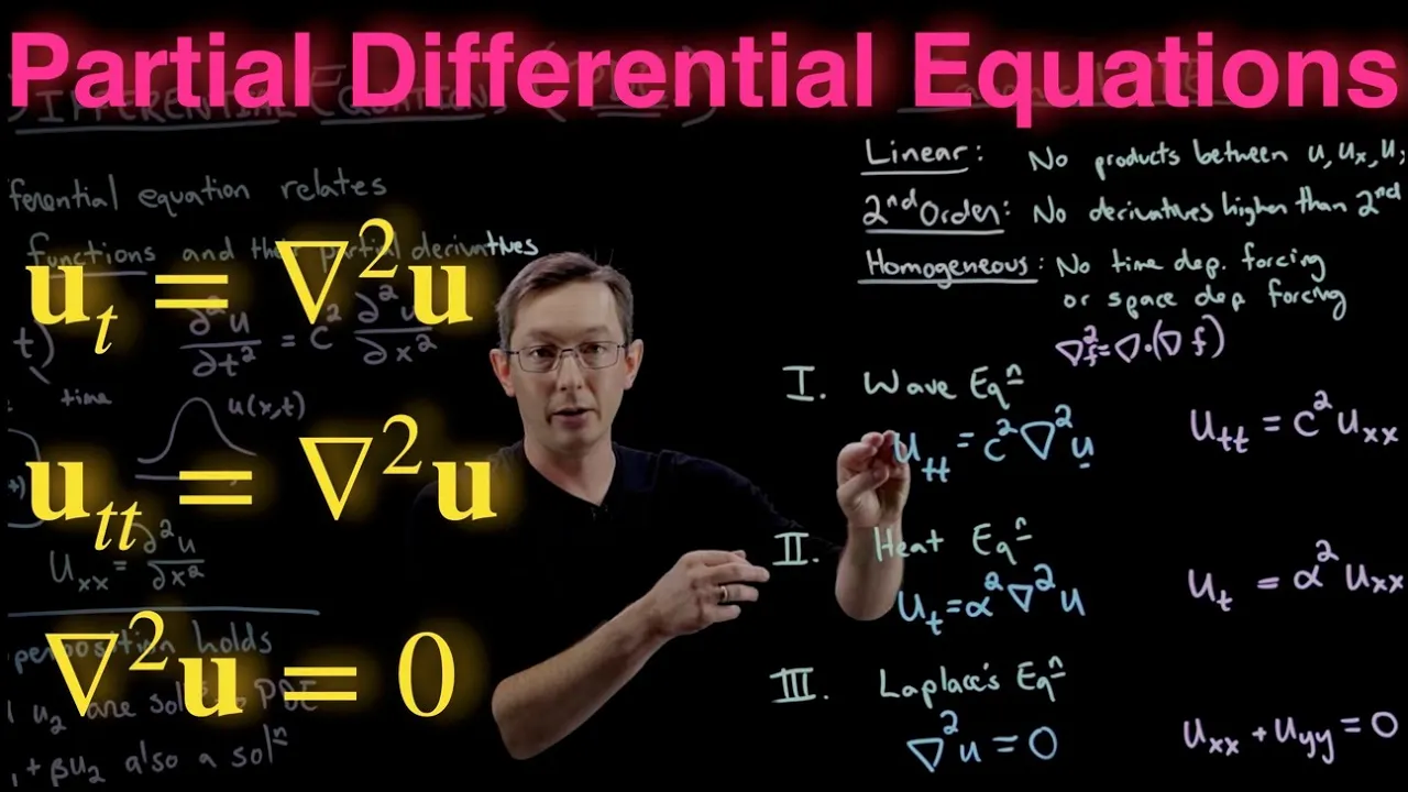
• Why this video: Steve Brunton ("Eigensteve") provides a high-level, intuitive overview of how partial differential equations describe physical systems changing in both space and time. This forms the essential mathematical baseline before diving into the specific equations of fluid flow.

Description and Derivation of the Navier-Stokes Equations

@LearnMechE11:17379,478

Description and Derivation of the Navier-Stokes Equations

The Navier-Stokes equations are derived from Newton's Second Law (F = ma) applied to an infinitesimal fluid element, expressing that the sum of forces (gravity, pressure, and viscous forces) equals the mass times acceleration on a per-unit-volume basis; the acceleration comprises local acceleration (time derivative of velocity) and convective acceleration (velocity gradient terms), with the final equations relating stresses to fluid viscosity through constitutive relations for Newtonian fluids.

@LearnMechE · 11:17

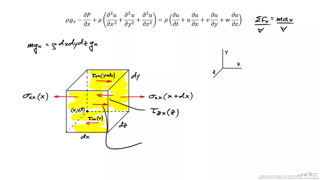
• Why this video: This video breaks down how the complex Navier-Stokes equations are derived directly from Newton's Second Law ($F = ma$) applied to an infinitesimal fluid element. It clearly demonstrates the balance of forces, including gravity, pressure gradients, and viscous forces.

Understanding the Navier Stokes Equations

@engineer_leo31:4957,341

Understanding the Navier Stokes Equations

The Navier-Stokes equations are derived from Newton's Second Law of motion by transforming particle-level equations to describe fluid volume behavior, incorporating temporal acceleration (rate of change of velocity over time) and convective acceleration (velocity transporting itself), with forces including pressure, viscosity, gravity, and other volumetric forces; these equations apply specifically to Newtonian fluids (like water, air, and oil) under incompressible conditions, and form a system

@engineer_leo · 31:49

• Why this video: A deep dive into the physical meaning of every mathematical component inside the Navier-Stokes equations. It differentiates between temporal acceleration, convective acceleration, and stress tensors, transforming abstract symbols into physical concepts.

Knowledge Checkpoint

• Understand the difference between an Ordinary Differential Equation (ODE) and a Partial Differential Equation (PDE).
• Explain the physical meaning of the convective acceleration term $(\mathbf{u} \cdot \nabla)\mathbf{u}$ in Navier-Stokes.
• Describe how Newton's second law ($F = ma$) translates to the conservation of momentum in fluids.
• Define the roles of pressure gradients and viscosity within a fluid element.

Module 2: Deep Learning & PyTorch Basics

This module focuses on the engineering tools necessary to build neural networks. You will master the fundamentals of PyTorch, from handling n-dimensional arrays (tensors) to structuring deep neural networks and configuring backpropagation loops.

Recommended Videos

The StatQuest Introduction to PyTorch

@statquest23:22205,214

The StatQuest Introduction to PyTorch

This StatQuest video teaches how to implement neural networks in PyTorch by creating a custom neural network class with weights and biases, performing forward passes to make predictions, and optimizing parameters using stochastic gradient descent with backpropagation to fit the model to training data.

@statquest · 23:22

• Why this video: StatQuest excels at breaking down machine learning concepts step-by-step. This video explains how to configure a custom PyTorch model class, define network weights, perform forward passes, and use the built-in optimization steps.

Neural Networks Pt. 2: Backpropagation Main Ideas

@statquest17:33732,041

Neural Networks Pt. 2: Backpropagation Main Ideas

Backpropagation optimizes neural network parameters by using the chain rule to calculate derivatives of the loss function (sum of squared residuals) with respect to each parameter, then applying gradient descent to iteratively adjust parameters toward optimal values; this process starts from the last parameter and works backward through the network.

@statquest · 17:33

• Why this video: Backpropagation is the engine that computes gradients for neural network updates. This visual explanation removes the complexity of the chain rule to show how the derivative of the loss function optimizes model parameters.

PyTorch Crash Course: Building Neural Networks in Python

@AssemblyAI49:54188,081

PyTorch Crash Course: Building Neural Networks in Python

This PyTorch crash course teaches the fundamentals of deep learning using PyTorch, covering tensor operations, autograd for automatic differentiation, building neural networks with model, loss, and optimizer components, implementing training loops, and creating convolutional neural networks with GPU support, data loading, and model saving/loading capabilities.

@AssemblyAI · 49:54

• Why this video: A comprehensive, hands-on coding tutorial on PyTorch. It covers vital components for PINNs: handling dynamic autograd (automatic differentiation), executing the training loop (zeroing gradients, forward pass, backward pass, optimizer steps), and defining custom layers.

Knowledge Checkpoint

• Create and manipulate multi-dimensional tensors in PyTorch.
• Explain the purpose of loss.backward() and optimizer.step() in the training loop.
• Build a custom multi-layer perceptron (MLP) by subclassing torch.nn.Module.
• Implement manual parameter updates and explain how backpropagation applies the chain rule.

Module 3: Introduction to Physics-Informed Neural Networks (PINNs)

Physics-Informed Neural Networks bridge deep learning and physical modeling. This module introduces the theoretical breakthrough of PINNs: leveraging automatic differentiation to compute derivative residuals, which are then integrated directly into the loss function to enforce physical laws.

Recommended Videos

An Introduction to Physics-Informed Neural Networks

@zara-dar07:0070,500

An Introduction to Physics-Informed Neural Networks

Physics-Informed Neural Networks (PINNs) are a type of neural network that incorporates known physical laws into the training process by modifying the loss function to include both data misfit and the residual of governing differential equations, allowing the network to make accurate predictions even with limited data by respecting physical constraints throughout the domain.

@zara-dar · 07:00

• Why this video: This video provides a direct, accessible introduction to the core architecture of PINNs. It clearly illustrates how the traditional data-driven loss is augmented with a "physics loss" component that penalizes solutions violating physical laws.

Physics Informed Neural Networks (PINNs) \|\| Ordinary Differential Equations \|\| Step-by-Step Tutorial

@elastropy10:3226,856

Physics Informed Neural Networks (PINNs) \|\| Ordinary Differential Equations \|\| Step-by-Step Tutorial

Physics Informed Neural Networks (PINNs) represent an innovative approach in scientific machine learning that solves differential equations by integrating governing physical laws directly into neural network training. Unlike traditional machine learning requiring extensive datasets, PINNs use differential equations and boundary conditions as their training data source. The methodology is grounded in the Universal Approximation Theorem, which guarantees neural networks can represent any continuou

@elastropy · 10:32

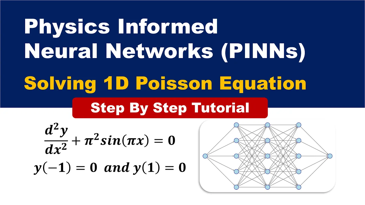
• Why this video: A clear, step-by-step mathematical demonstration of how a PINN evaluates a simple ordinary differential equation. It illustrates how network outputs are differentiated with respect to inputs to construct the physical residual.

Learning Physics Informed Machine Learning Part 1- Physics Informed Neural Networks (PINNs)

@juandiegotoscano_brown24:1941,718

Learning Physics Informed Machine Learning Part 1- Physics Informed Neural Networks (PINNs)

Physics-Informed Neural Networks (PINNs) are a type of neural network that incorporates physical laws directly into their training process by using the partial differential equation (PDE) as a loss function constraint. Instead of relying solely on labeled data, PINNs minimize a combined loss function that includes both the PDE residual (forcing the neural network to satisfy the governing equation at collocation points) and boundary/initial condition losses. This approach allows PINNs to approxim

@juandiegotoscano_brown · 24:19

• Why this video: This lecture covers the mathematical theory of PINNs in depth. It shows how automatic differentiation differs from numerical discretization (like finite differences) and how PINNs handle boundary and initial conditions as soft constraints.

Knowledge Checkpoint

• Explain how physics residuals are formulated as a loss function term.
• Describe the difference between automatic differentiation and finite difference methods.
• Understand how boundary conditions and initial conditions act as penalty terms in PINN optimization.
• Write down the total loss equation for a general PINN system.

Module 4: Coding PINNs from Scratch in PyTorch

This module shifts from theory to implementation. You will write code in raw PyTorch to solve physical equations. The practical focus is on the 1D Burgers' equation—a fundamental fluid mechanics equation combining non-linear advection and diffusion.

Recommended Videos

Introduction to Scientific Machine Learning 2: Physics-Informed Neural Networks

@scimlorg06:5718,927

Introduction to Scientific Machine Learning 2: Physics-Informed Neural Networks

Implementing PINNs requires defining scalar-to-scalar neural networks using chaining operations. The test function g(t) = u₀ + t×N(t) satisfies initial conditions structurally. For the ODE g' = 2πcos(2πt) with g(0)=1, the solution is g(t) = 1 + sin(2πt)/(2π). Training uses gradient descent on randomly initialized networks, minimizing the mean squared error between finite difference approximations of g' and the right-hand side of the ODE. After training, the neural network closely tracks the true

@scimlorg · 06:57

• Why this video: Demonstrates the programmatic structure of a PINN. It explains how to build custom training iterations that utilize scalar-to-scalar mappings and compute derivatives via PyTorch's torch.autograd.grad functional interface.

#105 Application \| Part 4 \| Solution of PDE/ODE using Neural Networks

@nptel-nociitm924001:0757,719

#105 Application \| Part 4 \| Solution of PDE/ODE using Neural Networks

Burgers' equation (ut + uux - μuxx = 0) is a fundamental partial differential equation used to test PINN methodology. It represents viscous fluid flow and combines nonlinear advection (ut + uux) with diffusion (μuxx). The initial condition specifies u(x,0) = sin(πx), and boundary conditions fix u at domain edges. Solving this equation demonstrates how PINNs handle time-dependent PDEs with both spatial and temporal derivatives.

@nptel-nociitm9240 · 01:07

• Why this video: Specifically frames the viscous Burgers' equation ($u_t + u u_x - \mu u_{xx} = 0$) within the PINN architecture, showing how this classic benchmark serves as a bridge between simple differential equations and complete fluid systems.

Gap Alert & Supplemental Exercises

⚠️ Practical Gap: The video pool lacks a comprehensive, line-by-line coding walkthrough for solving the 1D viscous Burgers' equation in raw PyTorch.

How to bridge this gap:

1. Independently search YouTube or GitHub for "Burgers' equation PINN PyTorch code walkthrough".
2. Ensure you understand how to use torch.autograd.grad(u, x, create_graph=True) to extract higher-order derivatives like $u_{xx}$.
3. Implement a custom training loop containing:
   • Spatial-temporal domain generation (x and t grid points).
   • A network predicting $u(x, t)$.
   • An MSE calculation combining Boundary Condition Loss, Initial Condition Loss, and PDE Residual Loss: $\text{Loss}_{\text{PDE}} = \frac{1}{N}\sum \left( \frac{\partial u}{\partial t} + u \frac{\partial u}{\partial x} - \mu \frac{\partial^2 u}{\partial x^2} \right)^2$

Knowledge Checkpoint

• Use torch.autograd.grad to compute first and second-order derivatives with create_graph=True.
• Construct custom training datasets representing boundary points, initial conditions, and domain collocation points.
• Write a raw PyTorch training loop that optimizes network parameters against a combined physical loss.
• Explain why the nonlinear advection term ($u u_x$) presents unique optimization challenges.

Module 5: DeepXDE Framework for Complex PDEs

When scaling up to complex geometries or systems of equations, writing raw PyTorch gets highly complex. DeepXDE is a high-level library designed specifically for scientific machine learning. In this module, you will learn to define domains, geometries, boundary conditions, and PDE systems inside DeepXDE.

Recommended Videos

DeepXDE Tutorial #1: DeepXDE Setup and Overview \| Physics Informed Neural Networks

@elastropy18:565,374

DeepXDE Tutorial #1: DeepXDE Setup and Overview \| Physics Informed Neural Networks

DeepXDE is a Python library that enables solving differential equations using Physics-Informed Neural Networks (PINNs) by defining the governing equation, geometry, boundary conditions, and training a neural network to minimize residuals while satisfying the differential equation and boundary constraints.

@elastropy · 18:56

• Why this video: An excellent starting point that introduces the structure of a DeepXDE program. It covers how to set up the environment, define a geometry (such as interval or rectangle), apply boundary conditions, and configure the training loop with minimal boilerplate.

Easy PINNS with DeepXDE: HEAT Simulation with Deep Neural Networks

@Dr.Mohammad_Samara11:238,468

Easy PINNS with DeepXDE: HEAT Simulation with Deep Neural Networks

Physics-Informed Neural Networks (PINNs) solve partial differential equations like the heat equation by training neural networks to satisfy both the governing PDE and its boundary/initial conditions simultaneously; the DeepXDE library enables this by defining the PDE, boundary conditions, initial conditions, and neural network architecture, then using optimization algorithms (Adam followed by L-BFGS) to minimize the loss function that enforces these constraints across the computational domain.

@Dr.Mohammad_Samara · 11:23

• Why this video: Walkthrough of a 2D Heat Equation setup in DeepXDE. It demonstrates the ease of defining initial values and boundary profiles using DeepXDE's functional wrappers.

DeepXDE: A Deep Learning Library for Solving Differential Equations by Lu Lu

@mlps-combiningaiandmlwithp289747:5020,011

DeepXDE: A Deep Learning Library for Solving Differential Equations by Lu Lu

Physics-informed neural networks (PINNs) embed partial differential equations (PDEs) into neural network loss functions using automatic differentiation, enabling mesh-free solutions to both forward and inverse PDE problems; DeepXDE is a Python library that implements this framework by allowing users to define geometry, PDEs, boundary/initial conditions, and neural networks through a modular API, with key features including residual-based adaptive refinement for efficient training and support for

@mlps-combiningaiandmlwithp2897 · 47:50

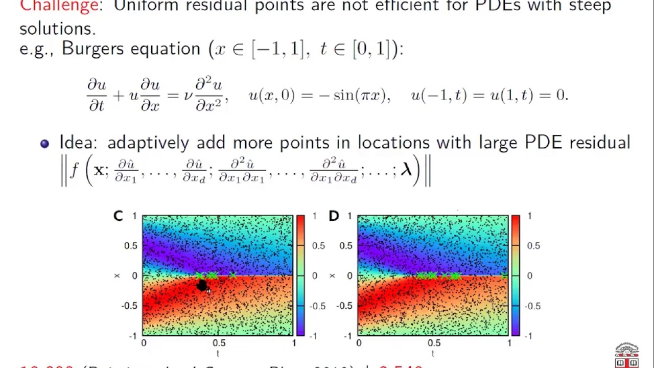
• Why this video: A comprehensive lecture by the creator of DeepXDE, Lu Lu. He details the architectural design of the library, how it handles complex multi-dimensional geometries, and how it utilizes automatic differentiation in backend engines (PyTorch, TensorFlow).

Gap Alert & Supplemental Exercises

⚠️ Practical Gap: The videos provide general setup overviews but lack deep, modular walkthroughs on defining complex boundaries (e.g., Robin, custom Neumann) and non-standard geometries in DeepXDE.

How to bridge this gap:

1. Search online or review the DeepXDE official documentation for: "DeepXDE boundary conditions and geometry tutorial".
2. Experiment with the built-in geometry classes: dde.geometry.geometry_2d.Polygon or dde.geometry.CSG (Constructive Solid Geometry) to unite/subtract simple shapes.
3. Write a script implementing Dirichlet and Neumann boundaries simultaneously on a custom 2D L-shaped domain.

Knowledge Checkpoint

• Initialize geometries in DeepXDE using classes like dde.geometry.Interval and dde.geometry.Rectangle.
• Define Dirichlet (dde.icbc.DirichletBC) and Neumann boundary conditions (dde.icbc.NeumannBC).
• Build a compile-and-train cycle using dde.Model, defining loss metrics and choosing optimizers (like Adam and L-BFGS).
• Extract and plot simulation results from the compiled model.

Module 6: Fluid Dynamics: Forward and Inverse Navier-Stokes Problems

The capstone of this curriculum. Here, you will integrate everything you have learned to solve the 2D incompressible Navier-Stokes equations. You will simulate fluid flows around obstacles (forward problem) and estimate unknown fluid parameters, such as viscosity, using sparse observation data (inverse problem).

Recommended Videos

CAII HAL Training: Physics Informed Deep Learning

@NCSAatIllinois04:362,071

CAII HAL Training: Physics Informed Deep Learning

This tutorial demonstrates solving Burgers' equation using DeepXDE. Steps include: (1) Install DeepXDE library; (2) Import matplotlib for plotting; (3) Define the viscous Burgers' equation with its PDE, initial conditions, and boundary conditions; (4) Load test data with exact solution; (5) Define geometry using Interval for 1D space-time domain; (6) Specify zero Dirichlet boundary conditions and initial conditions using coordinate-checking functions; (7) Create data object combining geometry, P

@NCSAatIllinois · 04:36

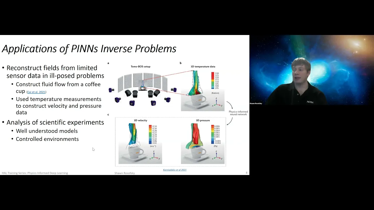
• Why this video: Demonstrates solving fluid-flow physics equations inside DeepXDE, guiding the learner through structured implementation phases from installation to variable definitions.

Maziar Raissi: "Hidden Physics Models: Machine Learning of Non-Linear Partial Differential Equat..."

@IPAMUCLA04:4120,439

Maziar Raissi: "Hidden Physics Models: Machine Learning of Non-Linear Partial Differential Equat..."

A systematic comparison positions PINNs alongside traditional methods: finite elements use weak forms and basis functions; finite differences discretize operators; reduced order models use interpolation; PINNs use automatic differentiation with gradient descent. PINNs gain significant advantages in high-dimensional problems due to the curse of dimensionality—traditional grid-based methods suffer exponentially increasing costs (10 points in 1D, 100 in 2D, 1,000 in 3D). Neural networks avoid this

@IPAMUCLA · 04:41

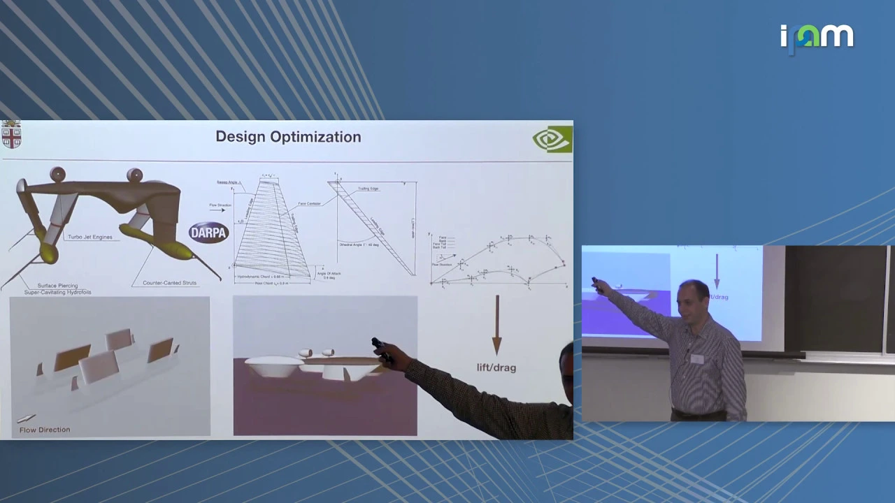
• Why this video: Dr. Maziar Raissi, a pioneer of PINNs, explains "Hidden Physics Models". He explains how neural networks utilize scattered velocity and pressure measurements to solve inverse fluid flow problems—discovering unobservable values like drag, lift, and viscosity.

Gap Alert & Supplemental Exercises

⚠️ Practical Gap: Complete coding implementations of forward and inverse Navier-Stokes equations inside DeepXDE are mathematically dense and are not fully walked through in the available videos.

How to bridge this gap:

1. Read through the official DeepXDE GitHub examples directory, focusing on the Navier-Stokes forward/inverse script templates (deepxde/examples/dataset/NavierStokes.py).
2. Search for the following precise queries on YouTube and Google:
   • "Solve Navier-Stokes using DeepXDE Python"
   • "DeepXDE inverse problem parameter estimation tutorial"
3. Implement a Project: Set up the 2D Navier-Stokes equations in DeepXDE: u_x + v_y &= 0 \\ u_t + u u_x + v u_y &= -p_x + \nu(u_{xx} + u_{yy}) \\ v_t + u v_x + v v_y &= -p_y + \nu(v_{xx} + v_{yy}) \end{aligned}$$ Using a sparse set of artificial velocity points, set up a variable `nu = dde.Variable(1.0)` and train the model to find the correct fluid viscosity.

Knowledge Checkpoint

• Code a system of coupled PDEs (continuity + momentum equations) inside DeepXDE.
• Configure dde.Variable instances to represent unknown constants (like viscosity $\nu$) for inverse parameter estimation.
• Train a PINN utilizing both PDE residuals and external data points (scattered sensor measurements).
• Evaluate the accuracy of parameter recovery in inverse problems relative to noise levels in input data.

Course Map

The following flowchart shows the recommended progression through the modules and dependencies:

Key People Index

• Dr. George Em Karniadakis (Professor of Applied Mathematics at Brown University)
  • Context: Broadly considered the father of PINNs. His research group published the seminal papers on Physics-Informed Neural Networks and DeepONets.
• Dr. Lu Lu (Assistant Professor of Chemical and Biomolecular Engineering at Penn State/Yale)
  • Context: Creator and main developer of DeepXDE. His contributions made physics-informed machine learning accessible to developers and researchers globally.
• Dr. Maziar Raissi (Assistant Professor of Applied Mathematics at CU Boulder)
  • Context: Lead co-author of the original PINN papers. He is a prominent pioneer in developing "Hidden Physics Models" that solve inverse fluid mechanics challenges.
• Dr. Steve Brunton (Professor of Mechanical Engineering at University of Washington)
  • Context: Renowned content creator ("Eigensteve") and researcher at the intersection of dynamical systems, fluid mechanics, and machine learning.

Final Self-Assessment

Complete this checklist to verify your mastery of PINNs for fluid dynamics:

• Explain how Navier-Stokes equations translate physical conservation laws (mass and momentum) into mathematical statements.
• Write a custom PyTorch class that inherits from torch.nn.Module and carries out a multi-layer forward pass.
• Write down the mathematical loss function of a basic PINN, distinguishing between the boundary loss, initial condition loss, and physical residual loss.
• Use torch.autograd.grad to manually extract first- and second-order derivatives from a PyTorch model's output with respect to its spatial/temporal inputs.
• Implement a raw PyTorch solver from scratch to model the 1D Burgers' equation ($u_t + u u_x = \mu u_{xx}$).
• Use DeepXDE to define geometric domains (including intervals and rectangles) and set up boundary conditions (Dirichlet and Neumann).
• Implement the incompressible 2D Navier-Stokes equations within the DeepXDE syntax.
• Explain the structural difference between forward PINN problems (solving PDEs with known parameters) and inverse PINN problems (discovering physical parameters from observation data).
• Run an inverse DeepXDE script that successfully estimates a fluid's viscosity parameter ($\nu$) from synthetic spatial-temporal velocity fields.