











![[한화에어로스페이스 고명석 박사] Physics-informed Neural Network-based Virtual Sensors](https://i.ytimg.com/vi/OycWHAw_hTg/maxresdefault.jpg)

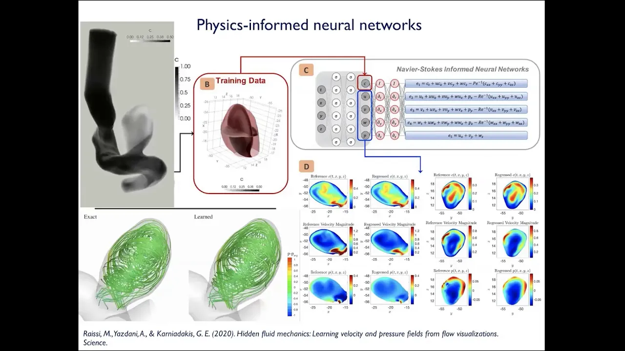


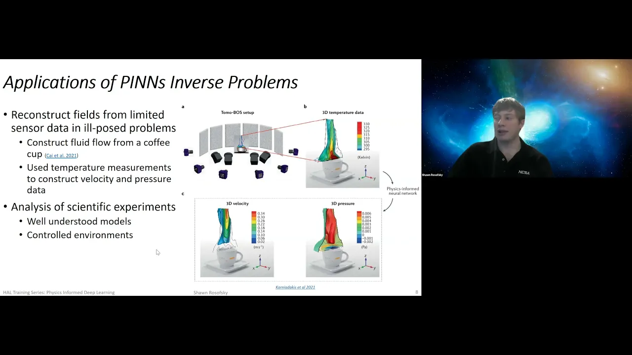
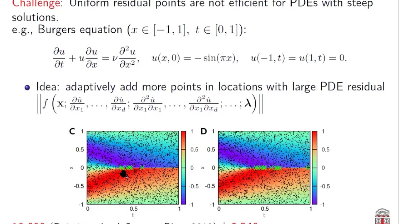



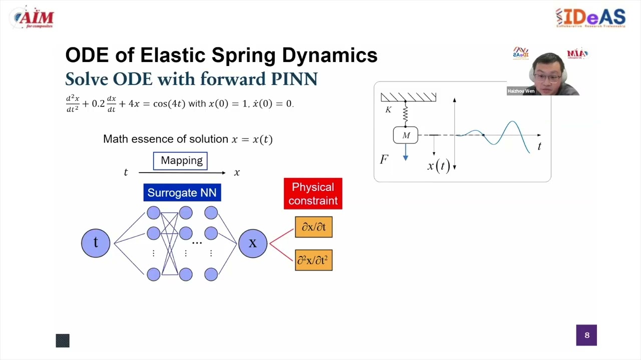
Physics-Informed Neural Networks (PINNs) are a type of neural network that incorporates physical laws directly into their training process by using the partial differential equation (PDE) as a loss function constraint. Instead of relying solely on labeled data, PINNs minimize a combined loss function that includes both the PDE residual (forcing the neural network to satisfy the governing equation at collocation points) and boundary/initial condition losses. This approach allows PINNs to approximate solutions to time-dependent PDEs without requiring the exact solution to be known beforehand, making them powerful tools for scientific computing and inverse problems.
Implementing Physics-Informed Neural Networks in PyTorch: PINN Tutorial
Added:Fundamental understanding of Partial Differential Equations (PDEs), including initial/boundary conditions and the physical formulation of the diffusion equation.
Proficiency in PyTorch, specifically in defining custom neural network architectures (`nn.Module`), configuring optimizers, and structuring training loops.
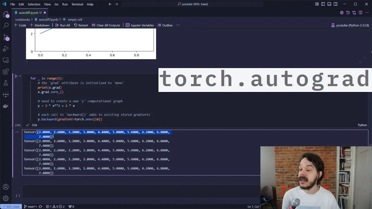
Core concept of Automatic Differentiation (PyTorch's `autograd`) for computing gradients, which is essential for calculating the derivative terms in the PDE loss.
Basic knowledge of calculus and numerical analysis to comprehend how neural networks can approximate continuous mathematical functions.
Solving inverse problems using PINNs, where the goal is to discover unknown physical parameters or coefficients from observational data.
Advanced optimization and loss-weighting strategies (such as learning rate annealing or self-adaptive PINNs) to address stiff gradients and convergence failures.
Scaling PINNs to complex, non-trivial geometries and high-dimensional domains using specialized frameworks like DeepXDE or NVIDIA Modulus.
Transitioning to Operator Learning techniques, such as Fourier Neural Operators (FNOs) and DeepONets, to learn mapping operators between function spaces rather than single PDE solutions.
41.7K views1Klikes24:19Original Release: 2022-04-10
hi thank you so much for watching my name is diego and today we will review how to implement a physics informational networking by church i uploaded a final code to my github and the link will be in the description of this video here you will find some other examples that could be useful to you if you're just starting in this field in this tutorial we will solve the digitization equation using a physics informal network as you can see this is a time dependent partial differential equation we'll be giving the domain the initial and boundary conditions and also the exact solution we'll be using the exact solution to evaluate our model and also to visualize the data however you will notice that we do not need to know this motion to solve this equation one of the key constitutes required to understand a physics informed neural network is that a neural network is essentially a function it's a function that has an extraordinary capability to approximate to any other function that is why they have so many applications in so many fields our goal will be to train a neural network that approximates to the solution of a partial differential equation a physics informal network is nothing more than a network that follows the rules of a partial differential equation but how do we make it follow the rules of partial differential equation well since a neural network is a function we can obtain its derivatives then we can arrange them to follow the structure set by the partial differential equation we'll tell this arrangement f now if our neural network approximates to to the solution of our partial differential equation well then f should approximate to zero and that is the condition that we will be using to train the problem we will evaluate our partial differential equation in a certain number of qualitation points inside our domain then we will minimize this new loss function related to it usually the training data is a set of points from which we know the answer from which we know the outcome and in our case this data is our boundary in our initial conditions so we will select nu points from a boundary initial condition and use them to train your neural net following the traditional means further that you may have seen it in another box then the total loss will be the sum of the loss from the boundary conditions plus loss from the partial differential equation we will install the python this is a library for design of experiments then we have to import a python for training the neural network we have to import map bloodline to plot the results and numpy to process the range to the data and here as mentioned by though or by doe we will use it for sampling and the lighting hypercube we will use that in the selected collocation points okay let's generate the data and also visualize the solution to know what we are trying to approximate to do that i'm including these uh functions that will help us with the plot please feel free to pause the video or remember that this code will be available in my github so let's just start defining a function for the real solution which is right here let's call this f3l we'll take x and t and we'll our solution which would be e to the minus t times times sine of pi x and yeah that would be now let's generate the data so we have x now search that link space we'll go from minus one to one oh let's make it turn three steps and also d to touch space zero from zero to one and just say 100 the steps will be your white this values the limits we're taking from the problem you can see here okay now let's generate a mesh now remember that we're working in a tree in the two-dimensional space so we need like a surface in order to obtain the result so to do that we just measure it and it works something like this starts that mesh grid it says xxxt now now let's evaluate our function which would be f3 would be to f real of x and d on the matrix and also let's plot the results in cloud 3d using the function we just created x t and y wheel now let's see what we have here yeah here we have the contour plot and the surface plot so this is the function we will try to approximate since we will be working with a fully connected neural network we cannot use the data we currently have without preprocessing remember that when we use smash grid we obtained a matrix for each one of the inputs i can choose now we will proceed with our column major flatten to take two vectors of twenty thousand point two two so to do that let's select it let's start with testing in group as this will use this one to avoid our model we'll start we will store both of them all the input variables so as you can see we have x dot transpose because we want uh a column major flattening we're going to flatten it yeah and then we will add an additional dimension that we will use a later year for processing we do the same here for the time i will do the same for the answer the only difference is that we're going to we are going to use the y realm that we just created a few minutes ago also it's it's at the lower bound and also the upper bound the lower bound will be nothing more than x test the first value and your upper bound will be the last volume so let's say let's say the let's set it with minus one okay now let's print the shapes that shape this is only for visualization processes we do not need to do that actually this last line of code actually and also let's print the lower bound and the upper bound we should figure together yeah you can see our x test store both of the both vectors for space and time of twenty thousand point each one and the answer only has one column also we have the maximum and minimum minimum volume for x which comes from minus one to one and from short time that comes from zero to one so remember that in a pin the training data data's initial condition the boundary conditions and also the coefficient so in initial conditions when the time equals zero then a a y equals sign of pi x and so it would be in the left edge and here of this graph so let's call that one left left x equals so we will save both a time and space so we will select them horizontally so it will be x we want uh the all the columns all the rows and terrain and for only the first column and yeah and we want to add the additional dimension and it would be none we will do the same for the time yeah we're good now let's focus left x that's why i'm sorry it will be torch that sine of y times of left x but what left x only take the x not both x and type right so it would be only the first column the first lecture that it's here so it will be all the color all the rows and all the differences yeah we're good now we need to include another thing which is this and a squeeze it's only to give it the right dimension it's similar to what this nun does actually i think it does seem uh now let's go with the boundary conditions in the boundary conditions it tells us whenever x is minus one or x is one then y is zero so we'll be here the top and also the bottom of this graph so let's go and say bottom x equals it will be the same as we have here the only difference will be that now we will be considering only the the last a the last row and all the columns and the same for the time plus row and all the columns remember this should be equal to zero so let's call this bottom y equals two torch that's zeros bottom x let's shape zero because we just want one dimension and also how many how many do we want we just want one column out right so we can let's see if we don't have an error view right so now oh i'm sorry here it should have been something like that yeah we're good i'm sorry for that let's go here and then let's go with the top top here we have a zero we just wanted one only the first column and yeah i think we're good to go yeah good now remember that we don't use all the data we just select certain points of the of the of the boundaries and the initial conditions so let's start starting molding all of them in a single array let's call this x-train equal storage that vertical stock but we'll save the left x the bottom x and the topics right we're good now let's do the same for the y so y train will be a left y bottom y and stop why look here well we're not good well i'm sorry it's be we stuck oh yeah i'm sorry for that yeah we're good now let's select a is just a certain number of points and let's say that our in u will be equal to i don't know what happens we're just going to like 100 points from the boundary conditions and let's see if that is okay um yeah i think the thing should be okay yeah if it's not then we can always go back so now let's see and to do that we select an index and now let's say random random it's random it's right here choice of extreme and we will select dot shape 0 because that it tells us how many elements it has so many points in here and we don't want to replace them raise equals false okay so now the extreme and let's it's i'm sorry for that extreme let's call this mu which is the one said we will use them to in one loss function will be or extreme the index and all the all the columns and for y train will be for the collocation points remember here we will be evaluating our pd we'll be using the platinum hypercube sampling that's why we needed that library by doe and we do something like this so enough strain and f will be the lower bound plus range so the upper bound like minus lower bound times uh the latin hypercube is space like happen to something i'm sorry and we want two columns and we want enough points and how many points we wanna we should do it with ten thousand points i think it should work well now let's go to the final step would be are we also going to evaluate the pde in the points that we selected off from our boundary condition so that's what we're going to do so it's starch dot vertical stock blood enough and also extremely yeah that should be good okay the last part here is to send all or for all data to the device which in our case would be a gpu but it could also be a scp okay so that's also pretty easy the only thing we need to do is extreme view equals extreme view forward yeah it should be the same for the nf nf and it should be the same for the y and can use this to evaluate attention and the last part here that we need to define is the it's a white hat and we'll call it f i'm sorry it will go in this will be george that's zero of x strain and f both sides epsilon f the shape zero remember the number of elements and just one column two device device remember that f should approximate to zero if it is working okay now that we have finished writing the code we can see what it does a python treats neural networks as classes and from this special class called in module first we initialize our neural network uh we said react said yeah the activation function will be the hyperbolic tangent also the loss function will be the mean squared error with the reduction we will try to reduce the mu uh this modulus helps us uh to change the architecture later if we want and we just input the python array with the layers and with the structure we want and the code does everything for us we initialize our weights with heavier normalization and we set the bias to zero and then uh we saw the forward pass which means manipulating the function which means passing through each layer and then activating it except the last layer because this is a great regression in our network yeah here we can see we have we also have here the the boundary condition the loss function for the boundary conditions you can see you input the x boundary conditions and the y binary conditions uh the loss function what it does is pass the boundary conditions through the neural network and compares it with a real volume this is the first loss and also the load of the partial differential equation and here it's what makes this neural network of physics information first we start by cloning in our volume to ensure that we will mess up the data when we work with it and also to activate these gradients so as you can see when we activate its gradients we enable the differentiation and that's what we we're going to use okay so we say f f equals to forward g so we pass the model then we take the first derivative using this long formula that i encourage you to review it and then we take the second derivative one thing to mention is that as we are inputting two variables this this variable will have also two variables in it so to select the first rivet respective time we will have to select the second volume and to select the secondary but respect to x we will have to select the first volume then we have away f f remember it's what we have here is this first derivative of the neural network respective time minus the second derivative of the learning with respect to the x squared plus this function that we have right here and this is exactly what we're the input that we're setting to uh this real value that you can see it here it's only to to give it the right dimension but it's mainly it's nothing out of this world and then you can see that we can pair the loss function f hat that should be zero because f if f should be close to zero if the on the network it's close to the partial differential equation solution so yeah then the total loss will be the loss function from both the boundary conditions and also from the partial differential equation okay now that we have weights in order we can start training let's start giving it some kind of architecture so layers equals and then array whatever we want let's say 2 32 64.
the only conditions are that the first one it should be two as we're going to do to space and time and then the last one is one because we're evaluating only why however we can change the the number of layers and the neurons from relay to pretty easy now let's clear physician from our network we just call it this way if it's fully connected network as that's how we define our class but yes now let's send on your network to device yeah we're good let's find our network to see what we have and yeah you can see the activation function the loss function we have the structure which is good okay now let's set the optimizer which should be equals to and we'll use the atom optimizer however we can try another one if we want torch dot option it's a library that contains the optimizers item what we're going to optimize the photometers become the learning weight let's set it to one to the minus three and numbers go out to false yeah and with it oh i'm sorry this should be something wrong yeah okay now let's start training therefore i in range also the number of steps iteration let's give it 10 000 you can give it more or less depending what you want okay now the loss will be ping that loss of what ex boundary conditions y binary conditions and xp remember that our boundary condition was saved here in the extreme in you so that's what we're going to do with extreme idea what else we will save or on our x-ray y training view which would be a white chinese y boundary conditions and also our xpd which would be x train enough or which will be your collocation points now let's a incidentally optimizer to zero nice into the back propagation so loss dot backward nice let's a update the values with the optimizer yeah we're good optimizer dot step and then let's print the values and to do that optimizer we will be using yeah we're good and today we'll be using the trade the testing data and it should be some somewhere around here yeah here's the testing data the only thing we have to do it is to send it to our device too that's what we're doing right now and then we're ready to evaluate and let's see if let's spread this everything in amount of time so let's do it 10 times so this is the way of doing that which would be 20 000.
the module white against that it's equals to zero then print here we will use with torch no graph and this will use as we just want to report the value but we didn't want to know three of the gradients as they should influence in the training process okay now the test loss should be equal to that loss the boundary king of boundary conditions because that's a traditional way of computing it against the data we know and of what of our x test and our why test in let's print the results which between what the loss which would be your training loss and also the test lost which would be let's see here training and also just right and let's save it something like that testing oh let's do it now okay that should work now okay the training you can see it will take a while and i'll see you receive you when it finishes training once we have trained our neural network we can start visualizing the results here we're using our physics inform neural network to evaluate the whole data and the code that you see right here it's only to reconstructive matrices remember this kind of neural network works with vectors not with matrices and here we are only reconstructing those those matrices these are the results from the physics information and these are the results from the reality you can see that they are pretty close and previously however if you want to improve the data to improve the results you can always modify the 20 parameters i'll say a number of layers a number of neurons in the learning way and you can change the optimizer and many other ways and that would be all thank you so much for watching it was my first tutorial so i hope you like
Up Next

11:23
Solving the Heat Equation with DeepXDE and PINNs
@Dr.Mohammad_Samara
8.5K views•2023-07-17

28:59
Physics-Informed Neural Networks for Scientific Machine Learning
@scimlorg
18.9K views•2020-09-10

4:55
HTTP Requests Explained: GET, POST, PUT, DELETE
@codecademy
103.1K views•2021-10-07

19:25
Enigma Machine Mechanics: WWII Encryption Explained
@JaredOwen
13.2M views•2021-12-11
Related Study Plans & Knowledge Roadmaps
Structured learning paths in Computer Science
computer-science
Building a Rust Debugger: ptrace, ELF & DWARF
01Systems Programming Foundations & Rust
02Process Control and the Linux Ptrace API
03ELF Layout: Inside Linux Executables
+ 3 more learning modules
38h6 modules
Explore Roadmap
computer-science
Container Runtimes: Namespaces, Cgroups & Go
01Linux Systems & Go Programming Foundations
02The Core of Isolation: Chroot and Filesystems
03Linux Namespaces: Process Isolation
+ 3 more learning modules
32h6 modules
Explore Roadmap
computer-science
Building a CHIP-8 Emulator: Rust & CPU Basics
01Computer Architecture Foundations (Bits & Bytes)
02Rust Programming for Systems Development
03CHIP-8 Virtual Hardware Specifications
+ 2 more learning modules
32h5 modules
Explore Roadmap
computer-science
Building BitTorrent: Go, P2P & Concurrency
01Go Fundamentals & Concurrency
02Networking Foundations & P2P Architecture
03Bencode Parsing & Torrent Metadata
+ 3 more learning modules
26h6 modules
Explore Roadmap