Physics-Informed Neural Networks for Scientific Machine Learning

[00:00:00]so okay now we know of machine learning as a method for function approximation right let's start to look into how we can use function approximation along with differential equations and this will start to be this bridge that we call the physics informed neural network which we will use to bridge between you know this field of scientific simulation and machine learning so this this this object what we'll be talking about right now actually has a formal name is called the physics-informed neural network so physics-informed neural network is where you use a physical differential equation as a regularization term inside of a neural inside of a loss function so let's actually see how you know when you when you pull this to its basic constituent parts how a physics-informed neural network is really a method for solving an ordinary differential equation um so this actually dates back um the the earliest i can find is actually 1998 where this paper there's this paper on using our artificial neural networks for def for solving ordinary differential equations and partial differential equations now the way to think about this is you know so a system of ordinary differential equations is defined by a this equation you know u prime equals f of ut where what i mean by prime is i mean the derivative with respect to t um right because u itself is a function of t this is kind of a shorthand um the way that this is a kind of shorthand for what people write as u prime um of t equals f of u of t t right and so the only thing that you can take a derivative with respect to here is this value t but because you kind of just understand that if t is changing because it's in the differential equation or if u is changing because it's defined by the differential equation then people generally omit the of t terms on the um on the u's so okay so we have this differential equation which just says when i take a derivative of u with respect to t i should have this function f um for all the t's in in some domain so here i'm going to say i want to solve this in 0 to 1 with some initial condition to solve this what we can do is we can say this is a function this is a problem where we want to find the missing function right what is this missing function well this missing function is the thing such that when i take a derivative of it it equals f right that is a missing function um right so we want to find we let our neural network you know n of t be something that we want our neural network to approximate u of t and what that means is that when we take a derivative of a neural network with respect to the input it should be equal to f of the neural network at that t right because th this is by definition what has to be true if this neural network is the solution to the differential equation right so that that that relationship is one to one if you find an object that satisfies that equation right that a derivative of it equals f then that object is the solution to the differential equation and so the problem of of solving this differential equation with a neural network is just finding a neural network such that when you take a derivative you get some you get this f right so this gives us so this gives us our loss function so what we can do is we can say here's my neural network with my current coefficients i can evaluate at a bunch of times t sub i you know you could have some crazy stress training strategy for how you come up with these t's let's just say you have some set of t's you want to use you what you do at those t's is you take the derivative of your neural network with respect to its input at those t's and then you subtract out f applied at the neural network right at the t sub i and you do this for a bunch of t's you square all the terms you add them together now why do you square the terms well you square the terms so that way all these terms are positive so that way every single time that you're that you have a difference between this value and this value right it keeps on adding to the loss and so um when your loss is equal to zero that means that the derivative of the neural network with respect to time equals the f evaluated at the neural network which means that it would be the solution to the differential equation right so if your loss function goes to zero here then your neural network is the solution the differential equation gives us a way to turn solving a ordinary differential equation now into one of these training problems um now what do we do about the the initial condition right because we don't just have this equation but we also have that we know what the value is at the start now the way to be able to handle this is to well one thing you could do is you could just say this is another loss function term right so if i evaluate my neural network at zero it better equal this term because we said it had to be true and if it's not true then there's a positive theorem and a loss function so let's make it true right that's one way to be able to enforce this um but normally enforcing things through the loss function is not as stable as structurally specifying it so what i mean by structurally specifying is this idea of generating a test function a neural network or you know this universal approximator which is in the space of functions which always satisfies the property that you have so to see what this looks like in action this is a very nice case to do this so here what i do is i can define g of t equals u zero plus t times the neural network at t when t equals zero then that means g of t equals u zero when t is non-zero then i have a universal approximator added to it right so this is a very nice way to be able to construct a a function a universal approximator which is always u0 at time t equals zero this is a universal approximator over the space of continuous functions right because this will continuously change away from u0 at around that point so yeah you have to prove that this is the universal approximator i'm not going to prove it here but you can kind of see how it's going to have that property right if you plug in zero for g of t you see a equals zero u zero you plug in any other t in there well then you have a neural network that can you know change it around and if a neural network can approximate any function then g of t can be anything it wants as long as it's not at zero and so this gives us this this structural property that if we use gft instead of the neural network directly then we have something that always satisfies the initial condition and so we can do the same process as above we we define a loss function such that g has to satisfy our you know g has to be the something that satisfies the differential equation but by using g we no longer have to have this this boundary condition term this um initial condition so let's actually code up the method let's let's actually do it so we can say well i want to have my neural network be something that takes in a scalar and spits out a scalar so here here's a nice trick for doing that so remember a chain is just something that calls functions right so you don't need to look at the neural network library for how to do these things you can use any function you want so here is what i want this to do is i want to have a scalar come in and i want to put it in an array and i want to do some neural net networky things right and then after i neural network around what i want to do is i want to you know i have one value but it's in an array i want to turn this into a scalar so i take the first value of that array this is equivalent to um doing this right so this is the neural network that takes in a scalar and spits out a scalar if you didn't use the library you can probably use you know static arrays and these kinds of objects to make it a bit more efficient but this is kind of a simple demonstration so this is this is the way to kind of hack the neural network library understanding what chain does to just you know make it be something that is now a scalar to scalar neural network so now what we do is i define this g of t right so g is this function that now this is my universal approximator that is something that has to be 1 at time t equals 0.

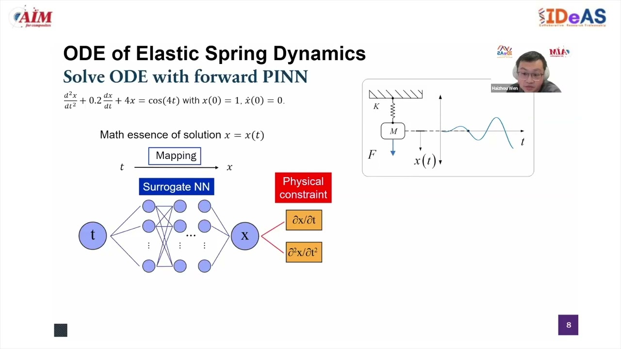
[00:09:01]so the differential equation that i want to solve here is i want to solve that u prime equals two pi t where u of zero equals one or u zero equals one so if i want to solve this differential equation how would i start to define this loss function well what i will do is i'm just using uh here i'm going to use uh finite differences for the for the derivative as a demonstration sorry so just just as a reminder this this term right here what this is doing is i perturb forward by epsilon then i'm subtracting the value and then i divide by epsilon right this definition of the derivative as epsilon goes to zero then um then this converges to being the derivative and so this is an approximation to the derivative at time t right why i chose epsilon to be square root of that square root of machine epsilon this is something that we'll go into later in the course so here um what i want to do is i want to what i want to do is i want to for t in from zero to one right so this is let me just let's just look at what this is right so remember this is a range object and so it's not as informative in that form but if i collect it into an array i can see all the different values and so this is you know starting at zero going by one f minus two so floating float32 values and going up by 0.1 all the way up to 1. so for each of those times what i want to do is i want to take my test function g i want to calculate its derivative at t and then i want to check it against the function f right so i want to check it against 2 pi cosine of 2 pi t and this should be equal to 0 and what i'm going to do then is i'm going to take the the square root of the square of that value i'm going to have my loss function be the mean of all of all these values so instead of just being the sum i divided by um the the number of terms so that way if i change the number of terms in my the number of t's that i'm evaluating at it doesn't actually change the relative size of my loss function so here's my neural network training problem what i want to do then is i want to say use gradient descent um my data so th this is a machine learning problem but i don't have data right so what i'm doing here this this is my little chi remember where i'm saying repeat empty data 5 000 times so you know it is training over data my data is just nothing and now i'm going to add a call back in here so that way it displays as it's doing the training process i want to do what i want to do in this here in this uh display is every 500 iterations i wanted to tell me what the loss is right so before we start what is the loss of my random neural network what how well is it doing it is at 4.5 f minus 6. i think let me make sure i take a completely random neural network so that way it's not rigged right so my average error here is 0.5 at each point in space now what i do is i take the as i run the training process right which will step 5 000 times and each time what it's doing is it is trying to minimize what the error between the derivative of g is from the evaluation of f where f is the differential equation term that i wanted to solve and after some computational churning which is a which is a rigorous term um then what we should see is we should get something that solves the differential equation so let's actually check our output here right so if we have this differential equation that g prime equals 2 pi cosine t well if we take the derivative of both sides then or if we take the integral both sides of our equation then what we get is g equals a constant plus sine of two pi t divided by two pi right that's just the integral rule and here we define c equals one y is equal to one well because that's what our initial condition was right so another way to think about the initial condition in an ordinary differential equation is that solving an ordinary differential equation is just taking the integral of both sides and you have a arbitrary constant that comes out the initial condition is the thing that specifies what that constant is so now let's let's actually plot this so if we take a bunch of different time points right we only trained on time points zero zero point one zero point two et cetera but let's plot on more time points just to see the regularity of our solution see how well it does and you can see over on the side from my notes while the plotting library is pre-compiling you can see that it very much matches the true solution right the true solution is a sine function that is perturbed and here what we have is the neural network is something that really closely tracks the sine function so this is a a way then to be able to train a neural network to be the solution to a given differential equation and now what we can start to do is we can start to use this idea to be able to augment loss functions with physical terms that are you know physically motivated by by these differential equations these physical laws and so let's let's look at doing a harmonic oscillator in form training um so here let me just kind of make sure that i get the plotting library set up because i'll be using it a bit here so let's assume that we are taking a bunch of measurements of some spring system let's actually take a look at this because i found a very pretty picture on the internet so you got to use it right so here we have a spring system and we as you move the spring away from it's it's from its steady state then what what you see is that you know so that this difference between this for between the spring from its steady state um it induces a force and that force that you get from the spring is linear right and this is called hooke's law and this is what everyone learns in you know first-year physics now let's this is true for a very idealized spring what are some things that we had to be true for this well you need to have that that you have the same mass throughout the spring um you need to have there's no frictions there's yeah there's a lot of assumptions that are made here in order to make this actually be the physical 101 version of the spring so the physics um 201 version of the spring has extra terms in there because you have deformities in the metal you have all these other things that can happen so let's actually let's let's assume that we have a real spring and our real spring has this extra plus sine term in there right because it's due to having some deformities in the metal um what we what we want to do now is we want to train a neural network that will be able to tell us what you know given an input f what force we would be expecting at a given point all right so we want to train a neural network to be the force function now given newton's law of motion right if this is our force then f equals m a and so if we assume mass equals one to be able to make our our units you know simple here um then what we have defined by this force equation is a second order differential equation um x double prime equals minus kx plus 0.1 sine of x right so let's let's take a look at this so here we can use the differential equation library to be able to we can use the differential equation library to tell us what the values would be if we were to solve this differential equation hopefully it's not going to have to precompile right now sorry about that and um and and so this this is what the solution of this spring looks like right so it's something that has a periodic motion just like the original spring but it has some kind of perturbation to the way that the the force is working because um it has a perturbation in there because um well we're we're assuming that you know maybe this part of the spring is less stretchy than this part of the string so as you start to stretch it around it doesn't uniformly always have the same force to go back so if you don't know this differential equation solving syntax don't worry we'll we'll be going over it in one of these future lectures so now let's actually look at what what the force is as we as we are going through the solution right so what what the solution is is looking at is that this is this is this blue curve is the velocity over time this orange curve is the position over time but what we want to learn is we want to look at the force and so what i want to do is i want to plot the force and i want to plot our data so let's say we we took measurements at you know every third interval um through time so here i'm going to take very precise measurements just to be able to build a plot and here i'm building the data set right so my data set is take the true differential equation solution and at these points you know zero point uh 3.3 6.6 9.9 let's say i have the the the actual value so no measurement error so i take the position out of there and i take the force out of there now let me let me plot what that looks like and here i show in the notes that um we didn't take it at very good spots right so um what what we get here is we get that are different you know the way that our differential equation is defined um makes it so that way the way that we we got our data we have forces at terms which are all fairly close to zero um so we didn't take very good measurements but could we still make a can we still have a neural network recover this function by using this data that's that's the first question asked right could could machine learning actually do this properly with this data set so we go okay i have my data set right i define my loss func i define a neural network i define a loss function and what i do with this loss function is i say well you know when here at each at each point in time i know i took a measurement of where the spring is i know what the force is there and i know what the velocity is at that point so what i want to do for my data set is i want to take the position i put this into the neural network right because the force is a function of position so i take the position i put in the neural net neural network this is a prediction of the force and i output the force right so i do this over every point in space i square it and this gives me my loss function with a random neural network this doesn't do so well and if i do gradient descent hopefully it does better all right so it trains a bit and now we can see how well our neural network does and we see that in some cases it can do okay right but doesn't really capture all all of the um all of the physics in there right it doesn't really capture what the peak is very well and the reason is because we don't have data at the peak so we need to have some way to be able to use the information that we know about physics to be able to supplement the data that we have from the physical system and so what physical information can we use well let's scroll up a little bit oh yeah we we mentioned that you know if we have a spring the first thing that you know you learn in your you know first physics course is hooke's law so you know that hooke's law should be you know for the idealized spring this is what you'd expect so let's use that as a starting point then right we can say hooke's law is approximately true right it's not completely true but it's a good approximation so we want to have our neural network be something that is use the data but kind of nudge it towards hooke's law you know let's let's do let's do a a mixture of being an idealized spring and something that matches our data points so the way to do this then is you know so so let's let's actually look at how close hooke's law actually gets on our system so if we actually look at a solution to the system where we say you know we drop that extra term it's not quite there right so it's not a great model but it's it's at least kind of a it's in in the right direction right it has the right structures so what we can do then is we can say well um let's have a term in our loss function which when that term is zero the neural network is something that completely satisfies hooke's law right it is something that solves the differential equation um and the way that you do that is precisely what we did before right where you know here we have a domain of times from we have a domain of times from zero to one and so here's a way to here i'm going to take a bunch of random values from minus one to one we have a oh and sorry we have a domain of positions where all these positions are between minus one to one so what i want to do is i want to take a bunch of random positions between minus 1 and 1 and evaluate the force at those points right so how do i do that well what i'm doing is i'm taking a random value from 0 to 1 i'm timesing it by 2 to get a random value from zero to two and i'm subtracting by one to get a random value from zero to one right i do that a hundred times so now what my loss function is going what i'm going to add is this this term for are you the solution to the ode that is hooke's law right and so that's what this this term does here so what i do is i want to loop over my random positions and for each posit in for each random position take the neural network you know the thing that comes out of it is should be interpreted as the force and see how close that force is from what hooke's law would give out right and on my random for my given neural network right now it is does not do very well so let's assume that you know i mean you did your physics first course right where you probably had to do this exact lab where you measure k on some idealized spring well on some spring in a lab and so let's assume that you know k right well we'll not you you could figure out k on the fly here but um let's start for now today by saying you figured out k from a lab so you can write down hooke's law here where you know what k is and we now have two terms for a loss function right we have one loss function term which is how well are you are you actually fitting the data that we need to fit and you have another term which is well we know physically that this thing should kind of be an idealized spring so here's the physical laws it should satisfy and what we can do now is we can say we we can put a weight in there we can say the we care more about matching the data but you should also understand this physical law if we don't have any data nearby and so this compose loss function is then the one that we want to satisfy and now we do exactly the same thing as before right so this is the loss function which has the universal approximator underneath it let's find the weights of the neural network such that we satisfy this loss function and when we do this we can then after training we can take all of the of all the positions right like a whole span of positions and then we can use that to be able to calculate what the force would be at each of those positions and now let's actually look at what we can use that to be able to look at what the neural network kind of is as a function and and plot it against the predicted force so right so this so this predicted force is what the neural network is outputting as what the force is and the true force is the force that comes from our differential equation and what we see here is that it's not perfect right but this is much better than what we had before what we had before was something that hit the data points well but it didn't really know more than the data points right and what we kind of fed it is well you should take into account how strings act generally because of this physical law and so what we what we get is we get a mixture between please match the data points and please be something that you know please match the data points and please be something that is kind of uses this physical law which isn't exact but it's it's something to kind of base your as a starting point right and the solution then is much improved and this this is what we're then calling this physics and foreign neural network because it is not the straight neural network trained from data this is a neural network that is trained from data that is mixed with a physical law and so this is really you know this is our first direction in scientific machine learning where you know what we motivated the way that we got here was that machine learning was not a process about predicting data but it's a process about learning arbitrary non-linear functions right and that is a very powerful idea right so there's so many times where you can you can specify a mathematical problem as find the function such that and machine learning is the process for finding said said function in very high dimensions and we can start to then if we understand it as just function approximation then we can start to use this function approximation in neat ways right so here we didn't have very much data but we can supplement that data by saying this neural network should be the object which also is the function that solves this ordinary differential equation so then we can you know put these ideas together and say i have this mechanistic differential equation for how a spring works use that idea plus this data and this weight between the if the physics idea and the data is what you should be neural network and then we can you know this this this way of doing it makes it a very well-defined optimization problem where we then find the weights for the optimization and train a neural network that can perform better than the data that we have on hand by using the extra physical information on hand this is the physics informed neural network and we'll be doing a lot more scientific machine learning digging into different methods but this is essentially you know deep learning in a nutshell and how we can start to move towards putting physical information into the way that we do deep learning