














![[한화에어로스페이스 고명석 박사] Physics-informed Neural Network-based Virtual Sensors](https://i.ytimg.com/vi/OycWHAw_hTg/maxresdefault.jpg)
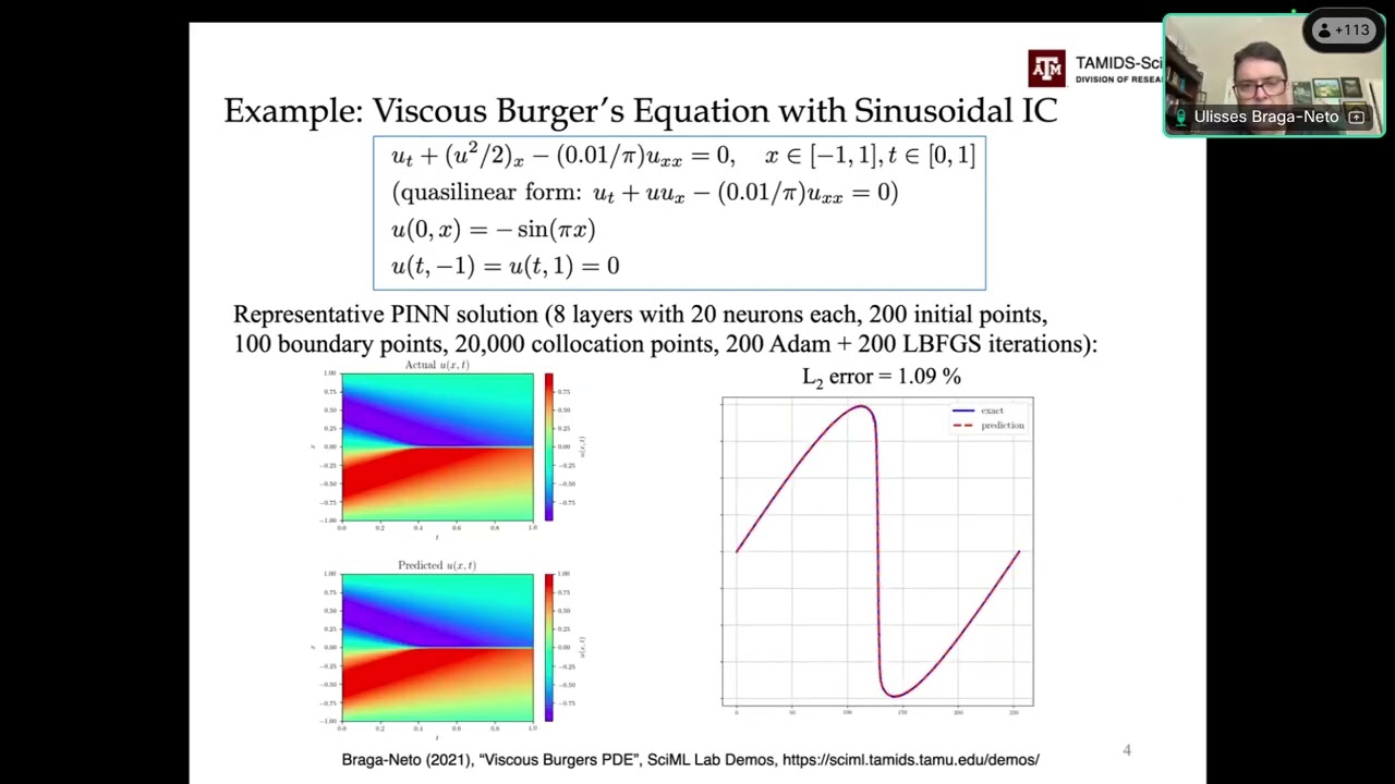
Physics-Informed Neural Networks (PINNs) solve partial differential equations like the heat equation by training neural networks to satisfy both the governing PDE and its boundary/initial conditions simultaneously; the DeepXDE library enables this by defining the PDE, boundary conditions, initial conditions, and neural network architecture, then using optimization algorithms (Adam followed by L-BFGS) to minimize the loss function that enforces these constraints across the computational domain.
Solving the Heat Equation with DeepXDE and PINNs
Added:Fundamentals of Partial Differential Equations (PDEs), specifically the mathematical formulation of the Heat Equation, boundary conditions, and initial conditions.
Basic concepts of Deep Learning, including feedforward neural networks, backpropagation, loss functions, and gradient descent optimization.
Intermediate Python programming skills, including familiarity with scientific computing libraries (NumPy) and deep learning frameworks (TensorFlow or PyTorch).
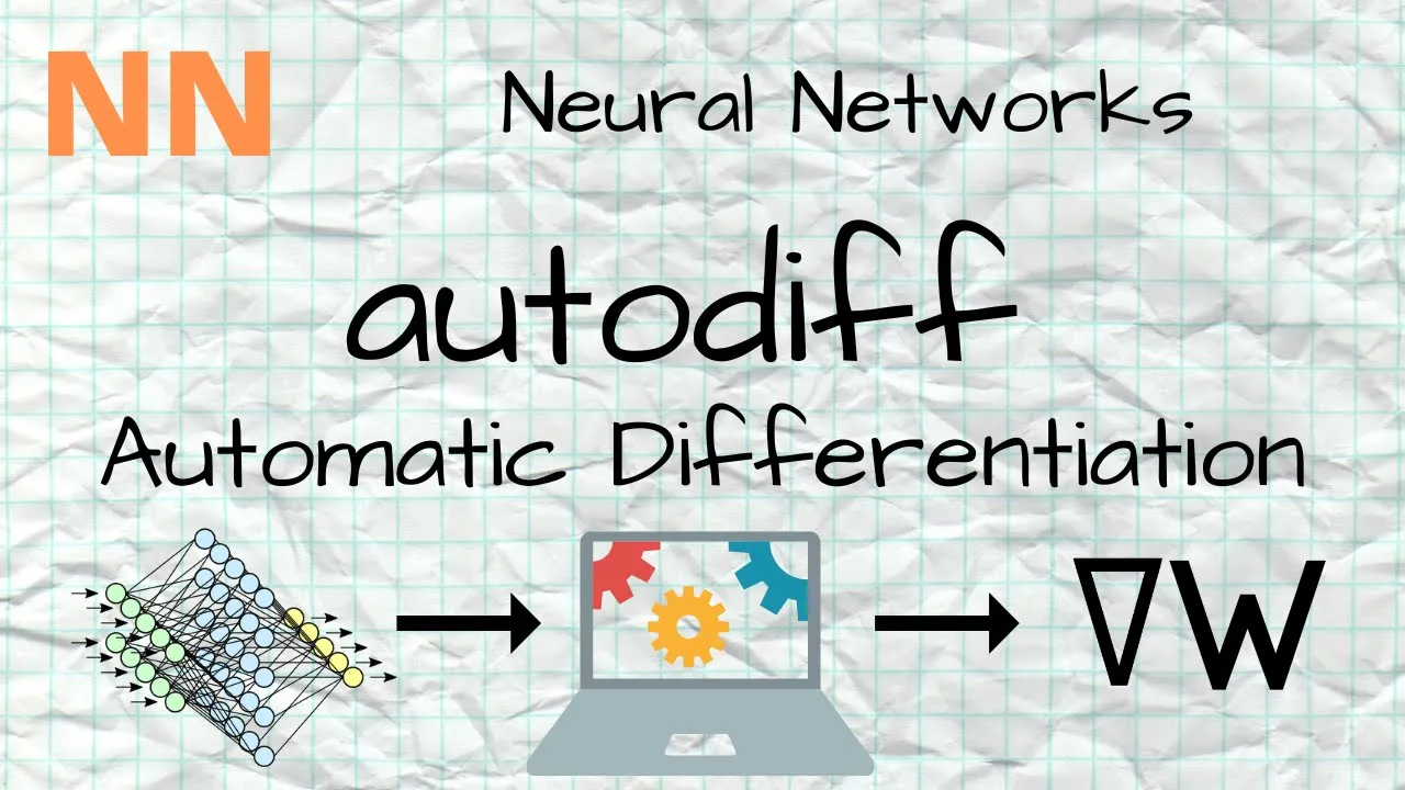
The concept of automatic differentiation, which is the underlying mechanism neural networks use to compute exact derivatives without mesh grids.
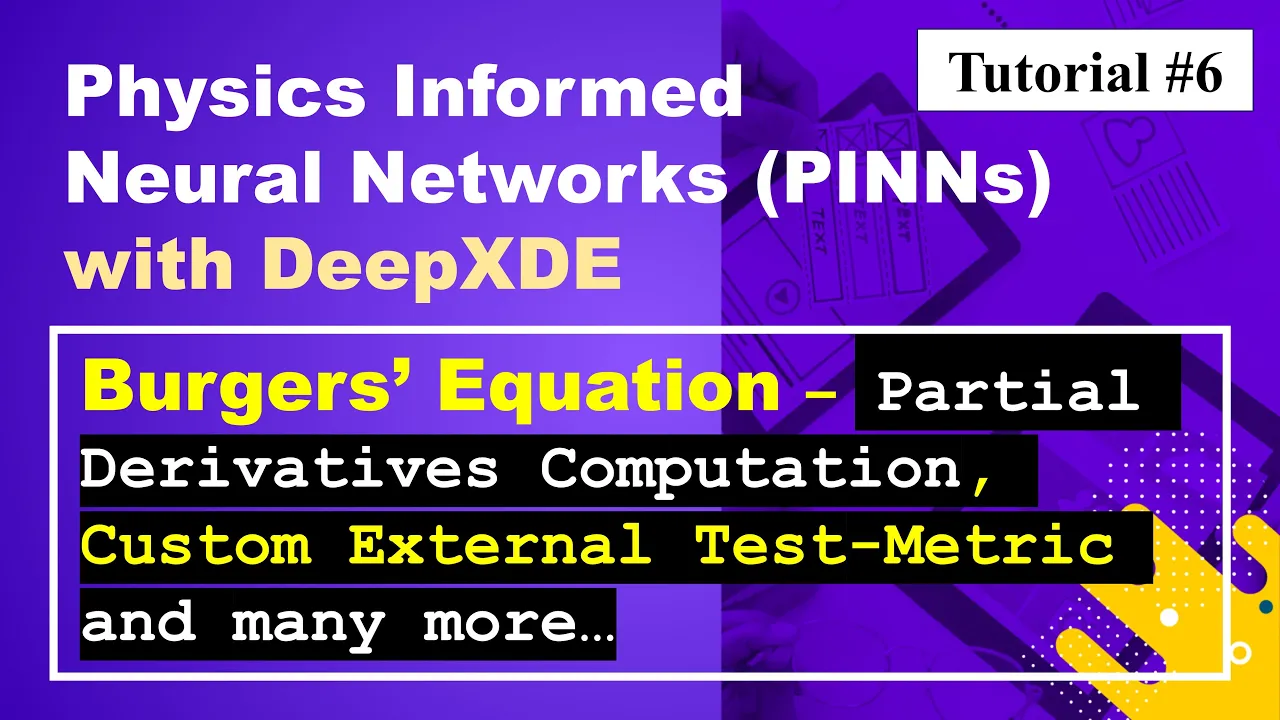
Solving multi-dimensional, non-linear, or coupled PDEs (such as the Navier-Stokes or Burgers' equations) using DeepXDE.
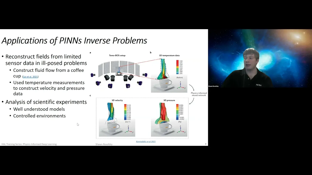
Applying PINNs to inverse problems, such as identifying unknown physical parameters or boundary conditions from experimental data.
Exploring operator learning and advanced neural network architectures, such as DeepONets (Deep Operator Networks) and Fourier Neural Operators (FNOs).
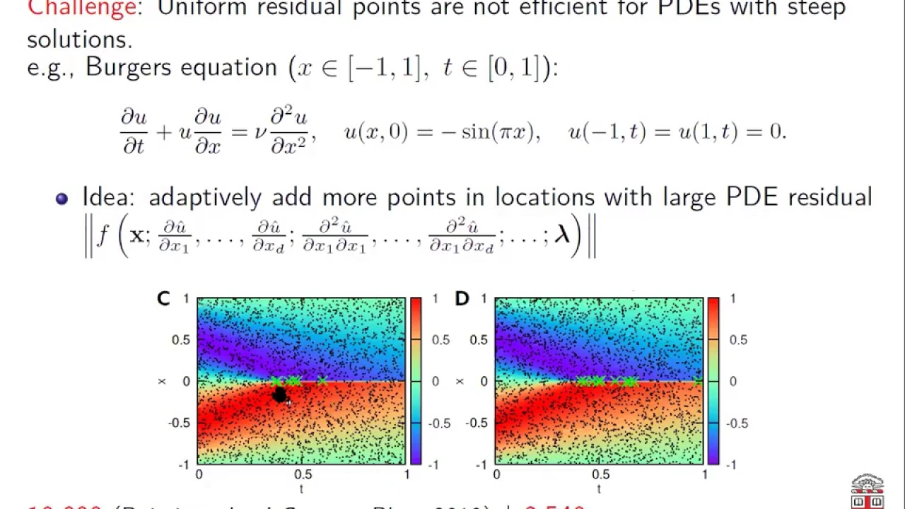
Implementing advanced training strategies for PINNs, such as self-adaptive loss weighting and residual-based adaptive refinement (RAR) to handle stiff gradients.
8.5K views210likes11:23Original Release: 2023-07-17
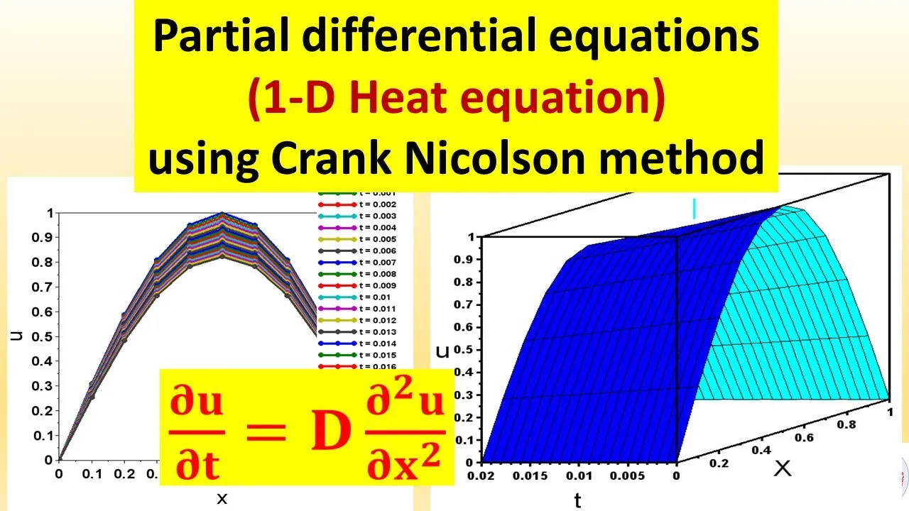
hello and welcome today we are going to explain the Deep xde library to solve the heat equation pde so in order to solve the heat equation first we have to import the Deep xde Library so we do that here as you can see import deep xde as DDE and we also you know import the the some back end which is here is tensorflow is also imported and importing a numpy the usual Library numpy as MP followed by that we have to Define the some variables related to the heat equation as we said just as a memorizer is the heat equation will have a function of d u over a d t a temporal derivation and of course the second derivation of U Square over well which is the second derivation of u 2 x here and of course we have the viscosity or the diffusion term the diffusion term or coefficient which is donated by X so we have to Define these three you know variables which is u t x and and we have actually K so it's four variables but of course U is the value that we are trying to actually calculate so let's do that so we have um in the first thing we have to do is the diffusion coefficient we have to Define its value and in this case is a 0.4 and we Define the limits of of of X and time so in this case we have to put l equals one and n equals one so the geometry interval is um from 0 to 1 and the time interval is from 0 to 1 as well now these both have to be inputted into gem time or geometry and time and we can put it in this uh in like in here so after that we have to define the actual pde and to define the actual pde we have to write a function the function will have two Imports X and Y and and what we will do is we will have we need to define the d y over DT the change of of course y over DT and the change of Y over x x of course uh Y in in our case is actually U so yeah we can change these namings but it doesn't really matter we can just use as s the most important thing is this function has to provide um this return which is the change of Y in respect to time minus the diffusion term and then the change of Y in this or the second derivative of y in respect to X here we can see d y over DT well he made it using Jacobian matrix and he well he used Jacobian metrics to get the first derivative and he used the Haitian or his Matrix to actually get the change of Y in respect to X and of course he returned it as the heat equation and as we can see here it's pretty much like similar to the heat equation which is we can see d u over d t is this one A K well it's here is a and d u over x x the second derivative of y in respect to X is is here so this is basically the heat equation now after that what uh what we need to do is we need to Define the boundary condition and the initial condition to define the boundary condition well with this also a function to do it but B what we need to understand here we have to Define it through equation or I think we can also Define it as a function but in our case we Define it as equation and here is we will take X which which has the value from zero to one this is the X going to change from 0 to 1 and the value will be 2 multiplied X so the boundary condition will be from the beginning it will be zero and at the end it will be two so it will start like basically like the S we have uh the beginning of um of x will start from 0 and 2x is zero and the boundary here will be a 2 so 2x will be two so these are the boundary condition now initial condition we also have to Define uh well based also an equation and in this case the initial condition is a sine wave and this sine wave well it's changed from zero to one and this is going to ex like the same way like we write equation and here is the X between 0 and 1 and then it has to be calculated through this equation and yeah this is how we Define the boundary condition and the initial condition now we take all of this and we put them into a function or or a value variable or compartment called Data now data equals when we add the geometry and time we add the pde and we add the boundary condition and the initial conditions are very important as as we need to use them to to get the data loss and here we will put the number of points that we need to optimize or to calculate using this Library so the inside the domain we will calculate 2540 points the boundary we will calculate 80 boundary components and initial condition we will use 160 initial condition points and this is just for evaluation the test we will use also a lot of points this is the same number and now after that now we are ready like our data is ready the geometry is ready the partial differential equation is defined what we need to do is we need to define the actual neural network and in deep X um well in deep dxde is is quite um sample to define the neural network um which is in our case this DDE what we already imported like which is the xde imported method here we have a DOT neural network and feed forward neural network now defining this neural network is very easy like we can see like we start from two variables in the input which is X and Y or in our case it's x and t time and the space and we have three hidden layers consists of 20 neurons and the output is one output which is in our case is U so we just get it like this and then we have the activation function is tan H and this is actually is for initializing the um the the neural network it's it's it's a way to initialize the neural network with a mean of zero this is just a method for initialization of the neural network now after here what we will do is we just Define the model which consists of the data we describe here and the network we described and then we well compile using Adam at the beginning which after that we start to train so here we use Adam with this learning rate and we train it for uh well 15 000 steps now it goes and keep training it and after that we compile using another method and this method is um is going to um tune the optimization get a better values it's called lpfgsb which is a it's it's kind of like a limited memory a Biden Fletcher glove for Sano algorithm is is this algorithm is actually used to tweak or to to get these small variables numbers to be a little bit more accurate and normal um neural network so we use this one so we start with Adam a little bit yscope and then we go back to the um more detail after that we will just we we get our loss we get everything done and we can see here the final losses and then we just print the results and here you can just save the plots you have and you can see the trend the test loss is pretty much you know go the same and here is the solution so you can see that at the beginning we have initial condition of the solution of course even here we have the sine wave and um we said the boundary condition is set from 0 to 2 and then everything will immediately diffuse from the sine wave or yeah not it will have some time but it will start diffusing from this initial condition to the our condition which is here representing a small temperature and higher temperature it it has to diffuse to this like with time the solution will be diffused to this linear uh you know like um shape so this is how we actually solve pde is using this deep d e the library and [Music] if you want to to know more about how to use machine learning for engineering applications please see the link
Up Next

24:19
Implementing Physics-Informed Neural Networks in PyTorch: PINN Tutorial
@juandiegotoscano_brown
41.7K views•2022-04-10

28:59
Physics-Informed Neural Networks for Scientific Machine Learning
@scimlorg
18.9K views•2020-09-10

4:55
HTTP Requests Explained: GET, POST, PUT, DELETE
@codecademy
103.1K views•2021-10-07

19:25
Enigma Machine Mechanics: WWII Encryption Explained
@JaredOwen
13.2M views•2021-12-11
Related Study Plans & Knowledge Roadmaps
Structured learning paths in Computer Science
computer-science
Building a Rust Debugger: ptrace, ELF & DWARF
01Systems Programming Foundations & Rust
02Process Control and the Linux Ptrace API
03ELF Layout: Inside Linux Executables
+ 3 more learning modules
38h6 modules
Explore Roadmap
computer-science
Container Runtimes: Namespaces, Cgroups & Go
01Linux Systems & Go Programming Foundations
02The Core of Isolation: Chroot and Filesystems
03Linux Namespaces: Process Isolation
+ 3 more learning modules
32h6 modules
Explore Roadmap
computer-science
Building a CHIP-8 Emulator: Rust & CPU Basics
01Computer Architecture Foundations (Bits & Bytes)
02Rust Programming for Systems Development
03CHIP-8 Virtual Hardware Specifications
+ 2 more learning modules
32h5 modules
Explore Roadmap
computer-science
Building BitTorrent: Go, P2P & Concurrency
01Go Fundamentals & Concurrency
02Networking Foundations & P2P Architecture
03Bencode Parsing & Torrent Metadata
+ 3 more learning modules
26h6 modules
Explore Roadmap