



![1) Adi Diferansiyel Denklemler : Dif. Denklem Tanımı ve Örnekleri [Ordinary Differntial Equations]](https://i.ytimg.com/vi_webp/BkVCADUC2wQ/maxresdefault.webp)




![[Scheme'22] Programming is (should be) fun!](https://i.ytimg.com/vi/2MYzvQ1v8Ww/maxresdefault.jpg)









![[ACM seminar] Speaker: Xueyu Zhu (University of Iowa), March 31, 2023](https://i.ytimg.com/vi/uAlUfv6FlIU/hqdefault.jpg)
![Physics Informed Neural Networks (PINNs) [Physics Informed Machine Learning]](https://i.ytimg.com/vi/-zrY7P2dVC4/maxresdefault.jpg)







Physics-informed deep learning integrates physical laws into neural networks by encoding partial differential equations (PDEs), symmetries, and conservation laws directly into the loss function, enabling models to solve forward and inverse problems with less data while ensuring physically consistent solutions; this approach uses automatic differentiation to compute derivatives and can be implemented using frameworks like DeepXDE, Modulus, or NeuralPDE, though each model must be retrained for different initial/boundary conditions, motivating the development of operator networks that generalize across multiple configurations.
Physics-Informed Deep Learning: PINNs Tutorial (CAII HAL Training)
Added:Fundamentals of Neural Networks: Familiarity with Multi-Layer Perceptrons (MLPs), loss functions, and backpropagation.
Ordinary and Partial Differential Equations (ODEs/PDEs): Understanding of differential operators, boundary conditions, and initial value problems.
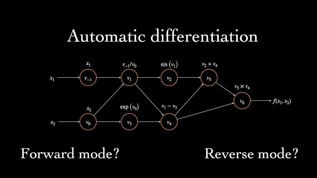
Automatic Differentiation: Concept of computing gradients of mathematical functions with respect to input variables using computational graphs (e.g., PyTorch autograd or TensorFlow GradientTape).
Basic Scientific Computing: General awareness of traditional numerical PDE solvers, such as Finite Element Method (FEM) or Finite Difference Method (FDM).
Advanced Operator Learning: Exploration of alternative architectures like Fourier Neural Operators (FNOs) for mesh-independent operator learning.
Bayesian PINNs (B-PINNs): Integrating uncertainty quantification into physics-informed models to handle noisy, incomplete, or stochastic data.
Domain Decomposition Methods: Studying frameworks like eXtended PINNs (XPINNs) to handle complex geometries and multi-scale physical domains.
Practical Industry Applications: Deploying PINNs for real-world engineering simulations, such as fluid dynamics (Navier-Stokes equations), heat transfer, or structural mechanics.
2.1K views79likes1:31:39Original Release: 2021-11-19
okay so hello everybody uh uh let's get started so today is our last uh tutorial or last last workshop uh in our series of whole trainings um we are very happy to have today uh uh shawn rasowski who is a phd student in the physics department and uh he will talk about physics informing deep learning in in his tutorial so he will explore how to incorporate physics into deep learning models with various examples ranging from using physics information networks to forward advanced problems to employee physics informant people diplomats or hybrid data and physics approach to problems and um so you know this is really an exciting area because uh the more sort of real uh real world constraints we can put into our machine learning models the more realistic these models uh will be and so this is kind of an important area to understand how exactly this can be done in the right way and uh how to take advantage of this so sean please take over from here hello um i am a i'm a fifth year graduate student at the uiuc department of physics and i work at the ncsa gravity group i'm here to talk to you about physics informed deep learning as part of the how training series and ex i'll explain how um how to incorporate physics information into deep learning models so first let me just give you a brief overview as to how this whole idea came about so deep learning has expanded tremendously in recent years this was fueled by many things including the availability of large data sets but improvements in hardware and the of open sourcing of large deep learning libraries such as tensorflow and pytorch however there are still cases where data is not always available the data might just be very expensive and or time consuming to produce however some of these cases you might have very good physical understanding of the system like uh scientific experiments and uh when you're designing hardware so one solution is to include the foods of our problem into neural networks and that allows us to train with much less data so how can physics help us well let's let's first introduce how neural networks they retain the bias of the training data for example gender bias in natural language processing of racial and age biases in image recognition we can remove some bias with data augmentation or simply just taking more data however in systems where we have well understood physics we can use physics to really remove lots of biases from our system and call and allow them to follow the true physics of uh the genome physics of the problem um we can do this by introducing by um by introducing symmetries conservation laws and in cases where they're known the partially differential equation describing the dynamics of the system so how do we code physics into neural networks well we do this by by adding our physical laws into our loss function this introduces soft physical constraints on the problem and this will continue to improve the more we train our network for for uh for problems with for physical laws that include derivatives we can um encode those derivatives by utilizing our deep learning frameworks automatic differentiation uh software this allows us to compute derivatives quickly and accurately moreover we can apply weights to the data and physical laws so that for for example complicated boundary conditions we can um we can we can improve our training moreover one couple things to note is that uh in many cases you need second derivatives so you can't really use reload activation functions which have a um zero um second derivative instead you've got um activation functions like uh tan h and um um gelu are more common in this field furthermore you make sure you really got to make sure that your data is normalized in order for these uh equations to work for this physics informed uh encoding to work so right here you can see a schematic of i would use encode physics into the neural network or barriers equation as you see we train the network to compute um this uh value u at all space and time with some data but we also add in these derivatives um into this expression which should be zero if this constraint is perfectly satisfied and we have a data part and a pd part our loss function we weigh each one and add them together so now let's talk about um specific physics and form neural network architectures um so traditionally pins physically form neural networks uh they're the most well-known type of physics-informed deep learning models they take uh space and or time coordinates as their input for time dependent problems and you can also add auxiliary variables um if it's useful in your particular case they output the pde solution fields at all over your specified input domain and you can also specify other outputs which is particularly useful in inverse problems so we train these networks by constraining the included physics and randomly sampling all of the domain to make sure our physics is satisfied all throughout the domain we can also add known training data to further ensure that the network obeys physical observations and one important note about pins is that each pin is only trained for a single case that means one set of initial conditions and boundary conditions and one set of pdes in other words we can't modify the source terms um you can see here this is how we use pins to solve the heat equation and we encode the physic the pde as well as the um as well as the boundary terms here we've got a dual boundary condition as well as a neumann one i can specify with different regions of the boundary now there are two classes of problems that pins are very are known for solving the first are forward problems where we solve the pdn on the specified domain later in the tutorials we'll look at using pins to solve a variety of forward uh problems we also have inverse problems um inverse problems is that when we're given data that raises unknown or partially known pde we can use that we can use pins to compute quantities of interest for example we can take we can compute a flow field from sensors at only a few locations moreover we can find um unknown pde coefficients from data um and we will later look at using at using inverse pins just to find the unknown coefficients of a learning system so here we see on this on the right this is the kdv equation uh in space center time for this particular set of initial and boundary conditions um what what's happening here is that the is that the pin is trying to compute these coefficients um for the effection term uux and this triple derivative term uh uxxx um and it does in two cases one with clean data and one is some noise and then you can see how then the pin tries to recalculate this field and you can see how accurate it is now for the app for some apple applications so uh for forward problems there are several use cases for pins over traditional pde solvers the first is being able to optimize over the auxiliary variables i mentioned earlier how we can have additional variables well one use case was actually showing how this can be done to optimize the heat sink geometry of fpgas where they use auxiliary variables to represent a bunch of different geometric configurations and they were able to optimize the particular configuration through using pins after training uh for quite a while and this to save them from doing a sim uh doing different simulations for each possible geometry then there are c then the other case is simulations of a very complex geometries uh one one good example of this is uh brain aneurysm blood flow so when a certain when um so for brain aneurysms you have you know the you can measure the inlet and outlet velocities as well you can uh maybe have some mri of the shape of the domain this is a very challenging problem for um for a traditional um pde solver to solve due to all this complex geometry however pins can solve it much more quickly and um and with reasonable accuracy as from the blood flow it can compute the velocity and the pressure as well as the flow stream lines with this information this allows uh can allow surgeons to to decide the best way to operate on this one a particular blood aneurysm and there's various treatment options um also one thing that really helped in this case was the use of transfer learning although pins only train for one case you can use transfer learning to significantly reduce the training time um now let's talk about applications to pins for inverse problems so one um one example is reconstructing fields from limited sensor data and ill-posed problems so we um so it was shown in uh diet all 2021 they will use these sensors to detect to measure the temperature coming out of the coffee cup now um and but then from that they were able to use those temperature measurements to construct velocity and pressure data using uh physics-informed neural networks and this um and this was um yeah and um and so and this is an ill-posed problem because we don't have really good initial uh or boundary conditions we just have some points during the data furthermore um in scientific ex various scientific experiments um if you have really well understood models and very controlled environments so it it would it might it's a good idea to try and use pins to try and look learn more about your about your um experiment from uh the known measurements so um now we're just gonna give a brief overview of some pin software first is deep xde which i'm most familiar with and we will use in our tutorials um we also have nvidia's modulus or simnet um it was for it's formerly known as simnet it changed his name to modulus um it's free but you need an nvidia developer package um if you have a couple more i'll just go to neural diff neural pde for those familiar with julio um as well um it also has this universal differential equations um has a bunch of examples using uh neural pde um if for those of you prefer deep learning with julia um yeah so uh one thing i should note is that there are limitations to pins mainly that they're only trained for a single set of initial conditions and or boundary conditions so you need to retrain the model for each new configuration therefore these pure pins make very poor surrogate models so later we'll look at using operator next for solving pdes with variable input fields however for now i would like to direct your attention to the then some jupiter notebooks where we will learn how to actually program pins and use it to solve uh forward and inverse problems now i'll put this link in the chat so everyone can uh who wants to can uh follow along and let me know if you've got any questions so far okay so um yeah so here's the github feel free to phone uh the repository and start getting working with these notebooks so the first notebook i'd like to go over is uh is this notebook burgers so this will solve the burgers equation using uh pins from the deep xde package um i'm just gonna give everyone a minute or two to if uh you're interested to uh to get your notebook set up and follow along if you are on hull you should be using this opence version 1.3.1 as your environment and you should top the notebook there should be this tip install mysq deep xde and that will install the deep xde library yes so the first thing we do is we need to install a package if we haven't done already all the notebooks should include this command i've already installed it um for my system so yeah so it should just say all the requirements are satisfied then um we're going to turn on this matplotlib notebook that will enable interactive plotting and here we will just import our libraries so here is the viscous verbs equation so here it is uh we see it um it's given by u d u dt plus u ux is equals 0.1 over pi uxx and it's got initial conditions and dear clay boundary conditions so here we have this so in this github repo we included the test data that has the exact solution so so that's just defining how we will load the test data so now let's get to how we do how we set up the pins for solving problems the first thing i'm going to do is to find my pde to the deep xd package we import it as dde it's got this very nice function um brad and um and then we can compute the first rows with jacobian and then this can just choose which x coordinate we um which uh we're knit which component so zero zero is the zero component y first component of x then d y d t um again zero component of y but the first component of um but the one component of x so this x here is position and time and then the second derivative where we have d y d x x and then we return this equation here um all right as notice in the chat i saw a question so it's as the difference between pins and ordinary dnn is only whether or not uh there is a loss is a pde loss uh term in the loss function are there any other differences um yes so um the so physics inform deep learning is when we include um information about the physics such as the pd loss term into our um into uh pd lawsuit into the loss of the neural network uh the pin is a network that computes the solution of a pde with input of space time and other auxiliary variables but the bit yeah the main thing about place and form deep learning is just including that physics term and the loss function okay so then um so now that i have defined the pde now i'll go ahead and find the geometry so here this is just a 1d problem from negative 1 to 1 and time from 0 to 0.99 so you just do this here it's pretty simple in the future examples i will go over solving things in more complicated domains um yes so just interval start point end point in 1d time domain start time end time and then then to combine them you just use this command dde dot geometry dot geometry x time so you can bind the space domain and the time domain and then we have initial conditions and boundary conditions so um dde package incorporates very many different types of boundary conditions um zero clay boundary conditions is um probably the easiest one to use so the way you do this is is you the first function that you add in is the geometry then you have the the second is you want to have a function that your input is your coordinates and that gives you the value of the of the boundary at the specified coordinate here it's just zero boundary conditions then finally this this func this last function here it tells you if the point is on the specified boundary now for just a single boundary um all you do is just have you can just have an empty first input this is your for this would be your coordinate and the second is if it is a boundary term so i if it's on the boundary of the domain um so and this form boundary is a boolean so this should this function should return uh true or false just to say all right is the given point on the boundary and if you've got various different boundary conditions it can say which boundary you want we'll see of some examples of more complicated boundary conditions later and the the initial condition here is given by this function d e dot ic so what this is is um the input geometry you've got then you've got um uh the points of the initial condition um so this is um negative mp dot sign that's just negative sign of pi times x uh the also i should note that uh that this deep xd package likes everything is uh as two-dimensional arrays even if it's just um a variable so this is a a um n by one array so that's that's why this zero to one is here and then um down here um you need to check just like you do it's just like the boundary condition the initial condition you need to check if it's an initial point so um again this would be a coordinate if we've got differential conditions for different places in the domain um but basically if we want to specify this format is true then um then we just um here is just is it a coordinate true or false and it will be input to our network let's go around these so then we can then we combine these together construct uh so this data term um here so dde.data so data gives us basically where we train the network the first term is the geometry the second term is the partial differential equation that we defined up here then we have the initial conditions and or boundary conditions the initial conditions are just treated as a type of boundary condition for the most part um then um then we control how many points from the sample so the first thing which we do is number of points in the domain um and then num points on the boundary and finally the number of initial points so i'm just going to run this runs instantly i don't know why it's yelling at me but i don't think it means anything the next part is how we define our neural network architecture so for most um for most pins we just use um uh simple um mlp architectures so um yes if you can just uh if you look at so we under gde.maps um yes it just basically shows how uh it just is um how we would different uh ways of desiring the um architecture so the first is just the first layer is just a list that should be that defines the different layers so this is two for the two input coordinates 20 20 times three so that's three uh we've got uh three 20 unit um middle layers and finally the output layers one output then we have an activation function and our initialization here the initial the activation function is tanh so just gonna run that runs pretty quickly and um yeah so now for to define our model which is a dd.model of net of the data and the network so pretty simple um yes i just want to go over exactly what everything is for the first example before we move on to some more complicated geometries so now we train the network so um i should note that the way um there are several ways to train the network so we actually train it twice here the first time with an atom optimizer and it's going to be for 15 000 epochs and then it's going to use this second optimizer um l bfgs b and this is a second order optimizer it trains more slowly but once we've got a model that has been pre-trained using atom you can only use a couple of iterations of this second optimizer and it will decrease the loss rapidly so now let's train it so i'm using a v100 single view 100 gpu on hull and uh yeah so i'm just going to train the network and it's training it from scratch and just need to wait a few minutes and we will uh while we're trying to network so feel free to ask me any questions while we're just training the network as you know that pins do train very fast i know that you need to train a pin for each case um it does it does sound pretty bad but uh it trains so fast that you don't really notice it the just minimizing the physics terms really does help and um yeah so now it's training with the atom optimizer so which now it's doing that uh secondary one with um this this uh l uh bf gsp yeah and then it now is finished so now uh dde is a bunch of functions that are able to bought its loss and um units i'm just going to go ahead and plot so as you can see here so this is its training and test loss very similar i should note that for that second so this is where the second optimizer came into play um it only evaluates on the test data at the start and end of its optimization process and you can see how much that second optimizer helped then these are the points in space and time so all right that's pretty good so how does it do on the test data uh 0.02 that's the error and now let's um let's see what that looks like uh so yeah so here is the um sorry it's the left what i so what i did here is i did um this is the x-axis is position y-axis is uh time is uh time and then we have the color bar so this is the exact predicted and the absolute air and you can see here the error is largest at the at the center right here by this shot from and now i'm going to show you um sort of animate what this looks like so we're going to see the exact solution versus the pin solution and you can see here it does pretty well and um um it does pretty well here although i have seen cases so sometimes what happens is that it gets the shock front off so what you can do um late again is that you can um add you can resample by adding more points by this shock to improve the performance of the network uh specifically at the shock points and um and we'll see how that looks and [Music] it's still training so yeah so it's just going to iterate through until the loss is um but the air all the max error is is um is greater than this value so yes this is just a way of improving the performance yes so what was really trained feel free to ask any questions you may have and it's going to try another iteration yeah so now it's finished uh updating so now i'll show the new results of the training so as you see it was adding points so um then i tried to reduce the air so now i'm just going to show you again the same thing so so unless so here the maximum absolute error is your point is around 0.06 and before and before we had the maximum absolute error of zero points around zero point or zero point two five so this shows basically um it can be helpful to add additional points near tough sections of the problem and then i'm just going to show you what the plot looks like here and you can see um yeah well both look cases actually look pretty good to me visually and yeah so this is the berries equation so now that i have introduced introduced uh deep xde i'm going to show you um how to um use deep xde to run more complicated geometries i'm just going to load the packages and here what we're going to do is solve the poisson's equation or an l shape so what that means is um so poisson's equation grad squared is equal to minus 1.
on the boundary we'll have to deal with boundary conditions but um but the the key is going to be our domain where it's going to be -1 to 1.
um and then zero to one and you'll and basically that means that the first quadrant is going to be empty all right so now what we do is first include our pde um again we should use this hessian function second derivatives the y is of um the x x and then d y d y y and then it's equal to -1 so here what we can use for the geometry is this polygon function this polygon function we can specify our vertices where they are so here 0 0 this is a two dimensional problem and you just do it on a different list so zero zero one zero one minus one negative one one negative one negative one negative one one and zero one and this will define our geometry there's different options this is a very generic option and then we define the boundary condition here we just have duplicate boundary conditions so we used to find this is a boundary located um it's from where it's located on the boundary and if it is x is going to be zero then again we're just going to do the same thing where we just encode the pde and boundary conditions and we can also include test cases and then we define the network architecture like we did previously and define the model here we then train our model and this is going to be again um we're going to use 50 000 epochs first with um with um atom optimizer and then with lvf gs and yes so let me know if you've got any questions as we train this model yeah so um yeah so this is again that it's gonna be two-part training where we first get get it around the right place with this atom optimizer and then we use this um lvfgs optimizer to further improve performance um yes so this um it's almost halfway done with this first round of training um and this and yeah so you can see that pins train very quickly um you can probably even train without a gpu although gpus obviously make it feel much faster again feel free to ask me any questions you may have um you all right so we're almost at the second round of training where we'll find the results yes so then this should take only a few more iterations and it should be finished and you notice that the loss function uh decreased by quite a bit here the second order option really does help quite a bit [Music] all right ah doesn't really take that many iterations usually so we should be about done with this [Music] and [Music] all right there we are we're done with the training there so um now i'm just gonna use this dde say that same plot function to um to plot my training loss and test loss as well as plot the points so you can see here this is the work of the first optimizer and then down here the second one so then we plot the coordinates and the solution and we just see it there so that's great but how does it compare the actual solution so i have included um in this github on the solution file we saw on it l-shaped.mpz and and now we'll just load the file and now let's see how fast it predicts this is going to be predicting the test points pretty much instantly and now i'm just going to compute the error about point one and i'm just going to get the points where um the test data set has some nand values so i just um go around them that's the part of the domain that is we don't want so i'm just going to now plot the results so here you can see from left to right the exact value the prediction and then the absolute error so we can see that the it's going to zoom out a bit so i don't need to scroll so yes so you can see that the um that the prediction is a little bit higher and right here is the absolute value of the error so um anything above zero tells you that there is um that there is some deviation not a certain direction but you just notice by this color bar that the prediction is um tends to be higher than the than the exact value um and particularly notice the air in uh near this corner here so i'm just gonna then uh do some uh surface blocks so that we can get a better views to the direction about see about the error to some shape in addition to color as well as the domain so yes so um rotate these there we are so yeah so this is i used to try um triangular triangulations so that to deal with this geometry and you can see this is the actual test values the the prediction and then the absolute error again right by the corner of the air is highest so like we saw in the bars example one way that we could probably improve this is is to again use that same refinement technique we will eventually add points there'll be lots of large air points particularly um you're by that corner so yeah so that's just some things to consider while training pens so then i've got the last pin example so this is going to be a very complex geometry where we've got uh we're going to have a geometry where we've got two holes we're gonna in the center of the domain so one so the domain is gonna be it's gonna be laplace's equation in um oops it'll be the fastest equation in um in x and y you can see here and then uh we're going to see if the um if on the boundary they are we're going to have dear clay boundary conditions and we're also going to have we're going to if if it's on the outside of the one of the holes it's going to have the the value of u is going to be one the other hole it's going to be minus one so the hole is going to have a radius of 0.1 we'll see better what that looks like i should note that this was a very this was originally from uh one of the issues in the repository um that inspired me to come up with this example so here is the pde so you can just compute the derivatives you're using this tf that grains as opposed to the um deep xd the jacobian function that's you can again it's all our differentiation so it all works then we need to for these more complicated geometries we're going to have to identify the boundary conditions so this boundary is just if it is on a boundary um that's what this tells you then if it's on the outer boundary what it checks is to see if the x squared plus y squared where x and y are between negative one and one if that is greater than point nine it it and it and it triggers this form boundary that and only in that case we'll um we'll will that consider that the outer boundary the cathode so the cathode is um is going to be locating the um the hole on the funnel um on the left side of the domain so basically if it's if it's greater than 0.9 um but less than but the x is less than zero then um it might it search and then it just plays it on the cathode and if it's a boundary greater than then 0 and less than 0.9 then it's an anode so then again if it is outer it's zero if it's cathode it's one anode minus one so again so that's just how to go through more complicated um boundary logic so one um so now i'm just going to introduce quickly how to combine different geometries in dxde so there are basically you do union intersection or difference union means if it's either in in g so if you take two geometries geometry one and geometry two or if it's in either of these two or in the union then it's part of the geometry intersection this is points in both geometry one and geometry two and finally difference exclude points from geometry which include geometry two from geometry one uh then just the difference so then the way we implement this so we define the radius of the circles point one in this case then the boundary the tool the full domains boundary is the rectangle then we have a disc for the cathode and disc for the anode then at x equals minus 0.5 and x equals 0.5 then we can make we can simply make this geometry by the boundary so geometry is the boundary minus the cathode minus the anode and then we just assign the boundary conditions for the outer cathode boundary and uh dear then the anode battery and then we just run that runs instantly and then we define the pde model and the net we define the number of points in the domain number points in the boundary and number of test points and again uh this network the the activation function and the um initialization and we then we get our model it gives us a warning because we can't use uniform points if we've got domain holes in it we need to use some random points that excludes places where we have the holes and again we'll use the same training configuration we had before we're going to train for 25 000 epochs and uh with the atom and then we'll train with this l um bf gsb for the secondary training and uh now i wait and feel free to ask me any questions while we're waiting for this to train um oh i should note one thing here that we i hadn't shown in previous cases which is this lost weights where it will weight the pde as one and then only each of these boundary conditions is 50.
because these boundary conditions are quite complicated we want to first want to first satisfy these boundary conditions and then we'll um then it will start then we want to satisfy the pe um otherwise uh you it would have issues near the boundaries so yes so now we just wait for it to train and you'll see because of the it does the boundary rates these loss functions for the boundaries tend to go faster than the loss function for the pde and um yeah so now it's 25 000 bucks and it's going to train for a bit more but the last time around this it was uh thou about a little over thirty thousand epochs in total so we'll just need to wait okay so again just um yeah you see because of the waiting terms that this this term here this pe term trains much more slowly than the others and there are other cases where this is useful in some cases where you've got like second derivatives the second derivatives um oftentimes have a lot larger value than um and then you say initial condition error so sometimes you might want to um to evaluate um higher weight on other terms like initial conditions as opposed to the pde um and that's with all different types of physical form deep learning just things to consider you got to play around with the weights all right so it's going to the end shortly of its first round of training so yeah so just um yeah so i hope you guys have a um let's just show you um uh how we can use deep xde to generate to solve bonds with very complex geometries and just how to combine different sorts of geometries and we'll yeah so hopefully we can students see the results and almost on the first round and zoom onto the second so now it's done the first 25 000 now it's going to try and use this other optimizer it means nvf again feel free to ask any questions you may have yeah one of the yeah so one of the things about pins is you really get it uh take advantage of these um this is kind of the second order optimizers where you can see that the atom optimum kind of slows down then we can really speed it up here this was a previous run i did um for the of this notebook so you can just see it was around uh order 10 minus 2 for the pde loss now it's 10 and -4 already after just a few thousand iterations and yeah it's gonna quickly come down yeah i should know i don't actually set the second optimizer's uh end time that it has some condition that so um yeah it usually only takes a couple of iterations and then it's um and it's really well optimized but i um yeah it was a little bit longer um so yeah so it looks like some non-trivial computations that need to happen there in the back yeah it should be almost finished um based on the last time i just finished here um yes so it's um the reason why this one in particular is taking so long is you need a lot of points near the boundary in order to make sure it actually computes everything i've discovered otherwise you just have massive errors that's um yes you just sometimes you want you need to add additional points here to complicated boundary conditions with these pens so unfortunately sometimes it takes a little longer um yeah and also the second order optimizer here although it trains quickly it's slower per step um that's why you want to use the second one but why you want to get it down with an atom optimizer and then this one here um this is much slower you just you just want to use it just to help it get a little bit further oh there we are finally it's finished yes so it's reduced it sufficiently and now we can look at these blocks uh again those those useful dde plotting functions so again you can see it goes down and then around order of 10 to the minus 2 and down all the way to 10 and minus relatively quickly and also it plots points so what you can see here is you see points for you can see what they actually look like so you've got you've got the geometry we've got um a square with two holes in it and you can see in your one hole it's around one and one minus one for the other hole so now let's see how fast that is to predict pretty much instantly and this was um what would consider the test data set um for the model so i um whenever i gave this uh this uh green uh test function here um that's same for the data it didn't train on so then you can use um um you can use the way you plot this is you you use a matplotlib's try function through a triangulation and make sure you mask out the pulse and that way you then get the predictions here i don't have the true solutions for this problem but these are what the network predicts and again you can see here this is a surface plot i think this shows it much better where and near the boundary it's one and either hole it's one or minus one depending on the whole and then it goes to zero um on the um near the outside of rectangle and this solves the fossil plate equation for cathode and anode on this boundary condition all right so that is last of the forward problems the last problem i want to show you for pins is an inverse problem so what we're going to do is we are going to look at the loan system which is a coupled system of odes determined by three constants we note that um so if we're going to ch for the defaults for this one it is um c1 is equal to 10 c2 is equal to 28 and c3 is equal to eight thirds um the end time to end is equal to three so this system is actually known to be chaotic uh for certain values um you can see i have a link to this with a b article for those of you following along um if you want to know more about lorenz systems so here i'm going to so here i want this for so that people can actually play around with this i include this generate train data function which will integrate this ode um given um so so it's um three initial conditions um your your pde coefficients end time um this dt is the integration um um time dt and then t skip is if you want to simulate um having less data than was used to integrate the pe i also have a body function below yeah so yes so you can feel free to play around with the the values um i should note that um again the system is chaotic around i guess the values i chose um i have found that there are cases where this problem will not converge so the issues i think are usually with a larger time scales um you want again you want to restrict your domain as much as possible this comes into just how pins like to be normalized so yes so what i'm going to show you is x zero is equal to one um x y zero is equal to minus one z zero is equal to two and a t skip is gonna be be 100 for the training so this is what it looks like in 3d space and then if you want to look at each important that's what it'll look like however i'm going to stop skipping and i just want to show you what this will look like if we go for a very long time and we get this very chaotic system here now again the system fails for these long times so it won't be able to do this so i'm just going to stick with the the shorter time scale but we're just going to what we're going to do is we're going to have the neural network be able to calculate this pde coefficients given the data so given this data we'll be i will teach the neural network to calculate those pe coefficients so the way we do that the first thing we need to do is make to ensure that these coefficients are set as variables so i didn't mention this before but deep xte can run on um different back ends high torch or tensorflow 1 or tensorflow tensorflow 2.
um i it's either it currently is running on tensorflow one or two i don't know for certain uh what's currently running on but um it doesn't really change much of the syntax but um so again so what we do is declare these as tf variables and that will tell tensor that will tell the um the code that the that it's allowed to change these parameters to optimize and that way we include these in our system is we make this the red system function of the input coordinates and the output um in our case um the time is our input output is x y and z and define and um the system is again shown here i want these two equal um if p satisfy these are zero and um yes so that is how we encode the pde but not the pde this is a coupled ode system here then we define initial conditions boundary conditions and um set the data so here it's pretty straightforward so the time challenge it's just the time domain which is just an interval um initial conditions are just the um initial chord uh just the initial value um i we get that we set those here and they're returned um as this y0 so um yes so um that's and that's how we set the initial uh positions and then the then we and we get the data by extracting the observations observe y 0 observe y 1 observe y 2.
and then um yeah so now that we've set those data we've got we've got to define our pde system so in this case geometry pde and then these are initial compositions or boundary conditions in this case our observations are treated as a boundary condition so uh here we have um so here we then just abandon point sampling the time domain only two points for each boundary and we anchor to the observed times that just gives us additional points so as many additional times we have it will make sure to sample those points and right and now we compile this is again define the network and just combine the data in the net and then here we add a callback for the variables so it will each time step it will save the variables to this file name so again so then when it every time we compute c1 c2 and c3 it computes that and also show the losses for those all right so let's just train the network okay so this is gonna train for sixty thousand epochs um i found that these networks will find well around between 20 and 30 000 epochs so you can see this is the previous case i've ran around 20 to 30 000 epochs is when it starts to really figure out the solution uh as to these coefficients and um yeah so then that is when um and then and then around 30 000 is when it will center in on the exact value so the losses so um yes so all these are different losses i'm not sure which refers to which some refer to initial condition some refer to the actual data but i believe the last three should be the loss the mean squared error of the three coefficients um and yes so now we just wait but i believe this one doesn't take too long as long as we get as long as it converges and we should know around 20 000 or so you should see the loss really decrease dramatically um yeah so we just wait yeah this one trains a bit quicker it's not very complicated no we don't have that many points for the boundary conditions yeah see the loss is pretty big right now but if it does converge which should dramatically decrease very shortly yes so yeah you can see it's gone down from 16 so that it's starting to really find the values and looks like this has converged and should around thirty thousand really start to find the correlation yeah you can see right now it's the air is less than one and yeah now it's just now it's just fine tuning itself and this is uh one of the real things that pins can do that a lot of other things cannot do which is just taking some data and be able to identify the governing partial differential equation i think that's really one of the most powerful uses of pins and the the time it takes is the same time i mean you saw this is quicker than it took to solve those pdes to the um this fine coefficients um again it's the same time it takes to train the footwork problem and now yeah now you're going to see it's really refining and if you are following at home you can uh feel free to play around with these um initial data generation parameters so these are just the initial coordinates uh it starts here in my case the end the end time be careful with this one that will change when it whether or not converge and then these three coefficients c one true c two true c show those um yeah so those are the coefficients trying to find and yeah so it's around 10 000 more epochs and then it should be finished all right it's finished so now let's see how it did this is my last run and this is my character that should be the legend supposed to be two columns anyway um oh there we are so yeah so now you can see we have um this time it took a little more than around more than 30 000 epochs and that really really quickly found the values of the coefficients and then it just fine tunes so now i'm just going to predict on the observations and um and just see what it finds and yeah you can see how well it does it pretty much exactly follows the pde and that's showing how to use pins for inverse problems and feel free to play around with them and that's the all i've got for pins i do have one other topic so if we go back to the slides um so now i want to talk about operator networks so i mentioned previously about the limitations of pins how uh pins you've got to train them and every uh another time for each and every problem um there we are sorry this video wasn't playing but um so now so one the thing with operants is they want to try and solve that issue by having a neural network train on given input fields this way the neural networks can learn variable initial conditions boundary conditions and or source terms the we need to in order but in order to do this we need to generate a data for many input fields however if we use uh physics information we should be able to improve the performance of the networks so i i've noted some very various examples of these kind of networks deep onex uh physics and form deep onex which is what i'm gonna do my tutorial on uh graph operator networks uh warrior opera networks and pinos um yeah so all these have links the papers for the slides for anyone who's interested these are to the top are showing how the network performs with different initial conditions the video so if i just restart the video i'll only play once but yeah you can see um the left is the ground truth the right is the prediction and you can see how it does for these different input conditions without any sort of retraining um this is with navier-spokesman number 1000 that's the top one below here is showing the vorticity i'm not 100 sure the exact problem that's being plotted but um but yeah so the difference here is that this one actually uses um physics information this one below and you can i mean this the top one i can see some differences between the ground truth and prediction um at least by eye i can't really see any differences although i don't i can't tell the color bar but anyway so now that i have um mentioned about operants let me explain some one of their architectures the physics and form deep bonettes which of the tutorial that i will be going over so deep o nuts um are can generalize software solutions including partial differential equations the way they work is they take two inputs this input field u which can be initial conditions source terms and or boundary conditions then it takes an input coordinate y which is space and or time and then it produces this operator g of u of y which is our pde solution and it does that by combining the branch net and the trunk net and just uh believe it just takes a dot product and then that's the then it gets the value the difference between you this the solution s and g of u of y is our loss in the classical d o nets the physics and form nets have been shown to improve performance while requiring less data the way we do this is we just incorporate the pde um into our loss as well as the initial and boundary conditions so then um all right that's good but how do we train these networks well i mentioned before we need to generate a bunch of use these init input fields and we can do this with gaussian random fields where we do this is we can use various kernels rbf or matern and this will allow us to obtain spatially correlated data we can then choose our length scale and that would be the length scale associated with typical standard deviations in our problem then we can expand these uh span this kernel and its fourier components in order to make the the uh venom field of a certain boundary conditions as you can see here we did this was using a matern kernel uh in 2d to to have it obey dual clay boundary conditions uh we then we will then have to run a simulation for each uh input field u to generate the training data we'll then sample the solution space during the training all right so that's good so let's go on to some examples so i'll present results for three of them a 1d diffusion reaction equation where this input field is our source term this described here in the equation this is the one i'll be showing a tutorial on i also have uh the 1d viscousberg's equation where u is our initial condition and we're using periodic boundary conditions here and lastly we have the 1d wave equation where u is also our initial condition all right so now let's look at some quick results the first is the diffusion reaction equation and um so those so the fusion reaction equation um given here we have the source term u these are two different source terms showing the exact solution s of x and t predicted solution and the absolute error then we've got the viscous burgers equation where we see we've got the initial condition um u of x exact predicted and the absolute error and if you just compare the absolute errors to the actual value you can see how it's bigger smaller it is finally we have the wave equation again initial condition exact predicting the absolute error one interesting thing about this case is that the errors actually propagate like a wave obeying the wave equation which implies a lot of the issues with the initial condition and that the initial condition just propagates um its error throughout the entire problem but still trying to obey the wave equation all right so now let's go back um to these uh networks you just click on the link so yes this one is this deep o net pi so unfortunately this problem runs on jacks unfortunately i could not get that to work on hull um so this one's going to be run on a different system which is um um bridges too so um yes so first things first again just we're going to get the plotting library and we're just going to get the various input imports so i'm just going to do a very quick introduction to jax so essentially a jax is just numpy on steroids what it is good at is it can map that numpy functions um to gpu and tpu devices with very slight differences it lets this r differentiation and with working with a level library like jacks it makes a lot of these fix and form deep learning applications pretty easy um so so yes so that's one thing you should know so i um so usually you want to make a lot of these base classes into separate functions um so i just have them here so if you guys want to refer back to them in the future both in these notebooks so these are just how we define different layers and jacks we've got mlp modified nlp and fourier feature network then this is a data loader where we just use um this is uh basically using the pi torch data loader to load in our data and then this is um going to be the actual base model so basically what this is is it will just declare the steep oh net as well as as well as defining the trainings the training procedure how we define the opera net and has uh place folders for the pde and boundary conditions initial conditions as well as ways it will calculate each of the losses as and then it will just just get training as well as saving and checkpointing um yeah but you um generally those would be in a separate file but it's here for convenience finally i have um how to this will show you how to generate random initial data with the rbf kernel and now all right so that's those are some of the all right so now how do we now we've got those uh out of the way so now let's talk about how we implement this diffusion reaction equation well the first thing we need to do is we need to we subclass that base network and we add in the pde and in jax you just take this grad function and you specify which argument on which you want to take the grad of first derivatives then the second derivatives like this so here it's just um 0 one two so uh d s d x x and we've got the boundary conditions and the initial conditions and those are um then uh here this is gonna generate this is a numerical solver for the diffusion reaction equation and then these the rest is just going to shape our data for the network yeah so it's a bit of complicated functions but essentially what this does is it this will just generate data for our network and have our network read it and then we define uh various parameters for our data set and so this length scale here i mentioned we can control i know the previous example for the diffusion reaction equation i had a length you have 0.2 i showed in the slides it's going to be 0.1 um and now i'm just going to show you what it looks like when we simulate a single uh training sample and then i'm just going to animate it so you can see what it looks like as it evolves in us as it evolves in space and time you can see how it just grows and yet the bit of an issue with um what's it called again how it was sort of the visualization but you're getting you get the idea then you generate the data and then we initialize our model so i know that some of the models have been around along this one takes about an hour to or so to run so i've already retrained the model so i just want to show you the results so yes so um so really quickly so this is on a i believe this is not a single training case uh no sorry this is 100 input samples right here and this computes the air and you see it's the mean error is uh 0.413 which is pretty low to me and this is what it lists the loss of liking training you can see the different losses and now you can generate a single test sample and make predictions so um so basically this is how you actually generate random numbers and it will always generate the same one for your random number key and then right there just make the prediction pretty much instantaneously and that would compute that error of that single term um order of ten to the minus three and i'm just going to show you what um sure the the exact solution and what the this deep opera internet predicts um it's actually the red line red dash line compared to the solid blue line the red dash lines are awkward and the network did not look good there try this again just so you can see what it looks like um as it will evolve it's going to reduce the size maybe that will help with some of the visual bugs and there we go and you see how it goes okay so then you can plot the the predictions and the true values and you can just see um again if you want to get more quantitatively where the area is a little bit of air in the um just um you see different regions here i have a function where you can plot all the various predictions so i did is i did 25 random cases and just showed you what they look like so you can get the source term exact prediction and the error and yes so you can see how well they perform so yeah so yeah so i just um i just wanted to give you um guys an introduction to a topic that's not just pin related but um in some maybe using physical form deep learning to look at another uh topic that can try and uh overcome some of the shortcomings of pins and yes so that's pretty much all all i've got so yeah so feel free to ask any questions you may have okay well so yeah if there are no other questions so sean thank you very much for for this tutorial this has been quite informative and very interesting we really appreciate you taking time for preparing this materials and making this available for us
Up Next
50:06
Hidden Physics Models: Machine Learning of Nonlinear PDEs
@IPAMUCLA
20.4K views•2019-11-12

30:57
Solving PDEs/ODEs with Neural Networks | Physics-Informed ML Tutorial
@nptel-nociitm9240
57.7K views•2019-05-06

13:03
Bypassing Tor Censorship: Bridges and Pluggable Transport Guide
@Coding_ForEveryone
397 views•2024-06-11

18:41
Neural Networks Explained: Math, Layers, and Learning Fundamentals
@3blue1brown
21.9M views•2017-10-05
Related Study Plans & Knowledge Roadmaps
Structured learning paths in Artificial Intelligence
artificial-intelligence
PINNs: Fluid Dynamics with PyTorch & DeepXDE
01Calculus & Fluid Dynamics Foundations
02Deep Learning & PyTorch Basics
03Introduction to Physics-Informed Neural Networks (PINNs)
+ 3 more learning modules
32h6 modules
Explore Roadmap
artificial-intelligence
Aligning LLMs: DPO, TRL & Custom Datasets
01Foundations of Python & Machine Learning
02Transformers and Large Language Models (LLMs)
03Aligning LLMs: SFT and RLHF
+ 3 more learning modules
24h6 modules
Explore Roadmap
artificial-intelligence
Federated Learning: PyTorch, Flower & Privacy
01Python & Machine Learning Foundations
02Deep Learning Basics with PyTorch
03Introduction to Federated Learning
+ 2 more learning modules
35h5 modules
Explore Roadmap
artificial-intelligence
Securing LLMs: Guardrails AI & NeMo Gateway
01Introduction to LLMs, Python, and APIs
02Understanding LLM Vulnerabilities & Threats
03Defending LLMs with Guardrails AI
+ 2 more learning modules
15h5 modules
Explore Roadmap