



![(New!!) [인공지능 특강] 18강. 신경망에서의 활성함수와 손실함수 | 은닉층에서의 활성함수 | 출력층에서의 활성함수 | 네트워크의 손실함수 | PART2.딥러닝 |](https://i.ytimg.com/vi/Uk7EZdITt30/maxresdefault.jpg)





![Deep Operator Networks (DeepONet) [Physics Informed Machine Learning]](https://i.ytimg.com/vi_webp/CDCyOHXDRcI/maxresdefault.webp)




![Rethinking Physics Informed Neural Networks [NeurIPS'21]](https://i.ytimg.com/vi_webp/qYmkUXH7TCY/maxresdefault.webp)


Physics-Informed Neural Networks (PINNs) solve differential equations by treating them as optimization problems: the neural network approximates the solution function, automatic differentiation computes derivatives, and the loss function combines the differential equation residual and boundary conditions to minimize via gradient descent, enabling automated solution of ODEs and PDEs without traditional discretization methods.
Solving PDEs/ODEs with Neural Networks | Physics-Informed ML Tutorial
Added:Basic understanding of Ordinary and Partial Differential Equations (ODEs/PDEs), including boundary and initial conditions.
Fundamentals of Neural Networks, including feedforward architectures, activation functions, and loss function minimization.
Concepts of optimization and training, specifically gradient descent and backpropagation.
Familiarity with Automatic Differentiation (AD) tools in modern deep learning frameworks like PyTorch or TensorFlow.
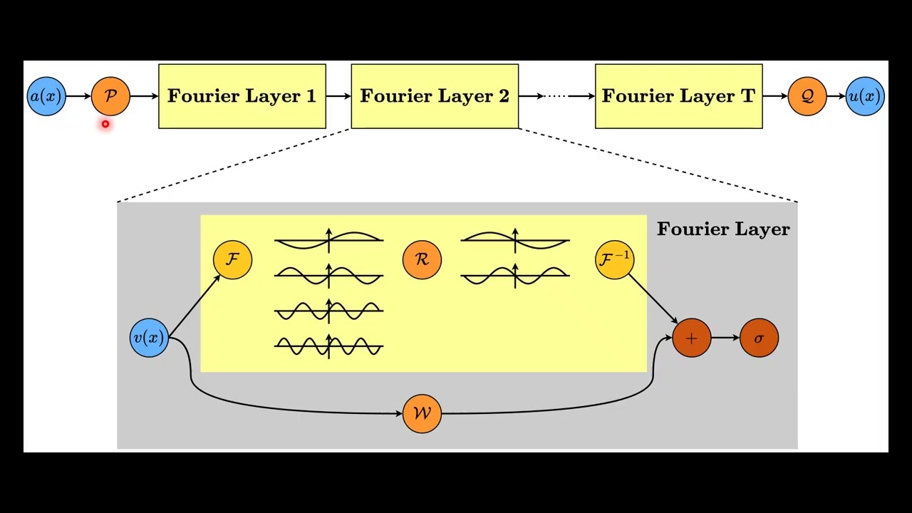
Exploring Neural Operators, such as Fourier Neural Operators (FNOs) and DeepONets, for learning operators instead of specific solutions.
Applying PINNs to inverse problems, such as parameter estimation and system identification from experimental data.
Integrating PINNs with traditional numerical methods (e.g., Finite Element Analysis) for hybrid physical modeling.
Addressing training challenges in PINNs, such as gradient pathologies, stiff differential equations, and multi-scale physical phenomena.
57.7K views1.5Klikes30:57Original Release: 2019-05-06
Welcome back, in this final application for this week we will be looking at something which is different from all the three examples that we saw before, this is the solution of differential equations using neural networks. So as you know in almost all of engineering and science most of us encounter differential equations in one form or the other. Now these differential equations can either be ODEs ordinary differential equations or PDEs.
Now here is the question can neural networks be actually used to solve ODEs and PDEs? Now unlike the other three applications I will not you know make a separate video for this just to describe the problem and then ask you to think about it because this is actually honestly it is a very very clever idea and it is unlikely that one would think of it on one its own. In fact it will look very very different from almost everything else that we have discussed in this course because you will not clearly see a training, set a testing set, or validation set, etc so please do remember this as I go over this example.
The idea behind this example goes back to a set of papers by Lagaris et al, this is late 90s, early 2000s if you just put Lagaris neural networks you should find these publications.
The application that I will be discussing right now is by a set of researchers from (())(1:52) et al, as you will see I will show you the paper shortly and this has just been published last year, so this is extremely recent. The reason for including this A of course is ODEs and PDEs affect us completely within engineering and science, B this is very different from the other applications that we have seen so far in fact this is not a surrogate model, okay.
So remember in the CFB video I had shown you how actually differential equations are discretized or using the finite difference method we kind of make an approximate equation. Now in this case we are not doing that you are using an entirely different method, you are posing every ODE or PDE as convert this into an optimization problem and you will see this extremely clever way of doing this, okay. Like I said the original idea was by these researchers and I would you know request you to look at it in case you are interested in this field I do think that this is going to get very important and before I describe the problem I would like you to I would like to talk a little bit about what the importance is.
So remember that when we were using finite difference method or whatever method that we had used to generate the CFD solutions this was still you know in the usual way.
Now in this case maybe using neural networks you can automatize the whole thing and the neural network can both solve as well as learn from the solution, so this is moving towards full automation of solving differential equations using neural networks that is first you solve it using neural networks and then you make a surrogate neural network for this original neural network this can look a little bit confusing but I do think that this is going to be slowly it will start seeping in into the mainstream of a lot of CAE solvers, so that is the reason for discussing this.
So let us take a very simple differential equation. So let us say I have the differential equation d square T dx square in fact let me change this variable to something else, let us call it d square u dx square let us say a du dx equal to b. Suppose you wish to solve this, you will also be given two boundary conditions without which you cannot solve this it is not a well posed problem.
So let us say u 0 equals u 0 and let us say this x lies between 0 and 1 and you have two boundary conditions. Now you can do this in multiple ways of course you can do this analytically, okay this equation is solvable analytically you would have seen this the second order linear differential equation or you can do this numerically using the kind of method that I discussed.
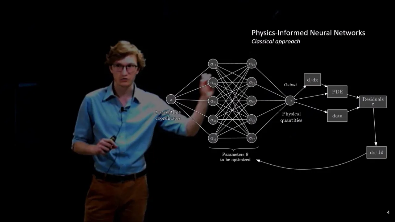
Now there is a third method that uses neural networks it is a clever method which is as follows. We assume that u is some neural network that takes in excess input and gives you as output, just to make this clear diagrammatically the neural network will look like this x this is the input of course typically we have a bias unit and then something happens here this is the neural network it could be in case you are getting unclear we can simply assume it is a single hidden layer and after all this you get u as output.
Now why is it possible? Regardless of which differential equation it is we know from the universal approximation theorem that I can always approximate the solution of u arbitrarily closely by a neural network, okay so because that is possible I can always assume that u is some neural network of x, okay. Now how does that help us? It helps us because suppose I postulate, so suppose I decide you know just like we did with the you know theta BMX example I take x let us say I put in 10 neural network or 10 neurons and here is u, okay.
Whenever we do this we are actually writing a full functional form for u, how is that so? Let me take a simple example let us say x is there and for now I am going to forget the bias unit, let us say there is a hidden neuron A, let us say this is my simple model and then I have u, okay. So what this says is a 1 is of course sigmoid of some w, x and you is let us say this is a linear layer and this is sigmoid in it and u is some other w 2 times sigmoid of w 1 x.
Now suppose I want du dx I can actually calculate this analytically I can write this as w 2 sigmoid prime w 1 x times w 1. Similarly you can calculate d square u dx square etc that is all derivatives this is the key point all derivatives of u with respect to the input x can be found. Now you might think that this is possible only because I had a single hidden neuron, what if I had 10 hidden neurons or worse still what if I had multiple layers of hidden neurons?
Okay, even if you have multiple layers of hidden neurons through backprop you can always find out d of the output with respect to d of the input just like we did d of the loss function with respect to the weights, you can similarly find out using the same backprop idea this is called automatic differentiation, so same idea you use output with respect to input in fact tensorflow has inbuilt functions that do this, okay I will show you the function I will show it to you from the paper you know how they actually did it.
So the point is this the moment you give a neural network we can find if u is a given neural network of x, we can find u prime of x which is du dx, u double prime of x, etc okay. Now this makes things easy for us, why? Because now instead of saying I am solving this equation I will pose the problem as follows d square u dx square let us call since this is an approximation we will call u hat just like we did y and y hat, so the original is u, the neural network predicts u hat, so what u hat do we want? We want u hat to satisfy del square d square u hat dx square plus a du hat dx minus b equal to 0, but obviously it is not going to be exactly 0, so what do I do?
I square it and say minimize, okay. So this is an extremely clever posing of the problem, instead of saying I solve d square u dx square plus a du hat dx minus b equal to 0, I say minimize this and obviously the actual minimum will be only for the exact solution because that would be 0. Now what you will get in practice of course is something a little bit closer to 0, but it will not be exactly 0 because our neural network will in general not approximate this you know not not get the exact solution, okay.
Now this tells you that this is the cost function that you have to minimize and the moment you put in the neural network it can for a given w let us say you initialize with some w’s let us say w 1 w 2 in the example that I gave, you put that in calculate this from the neural network because w 1 and w 2 are given you can actually do forwardprop calculate this, calculate this, calculate this try and minimize, do gradient descent this is our new cost function.
But if you have been paying attention so far you will notice that this is not sufficient because we have this condition also, what do we do about this? This will just satisfy the ODE but it will not satisfy the boundary conditions, turns out that is straightforward also, all you need to do is add that also to the cost, how do you add it? You say u hat of 0 remember if I give 0 as input in this neural network it will find out a u hat minus u 0 which is supposed to be the exact solution plus u hat 1 minus u 1 square, so this total thing all put together is our loss function.
Please think about this, this is an extremely clever posing of the problem so that differential equation and the boundary conditions have all been put together as a single optimization problem, so the ODE has now been converted to an optimization problem and after this it is simply a solution, okay so how will you solve it? You try various values of x that is let us say you have 0, you have 1, now as it is posed for each x, so you will put x equal to let us say 0.1 run this that will give you a residual or that will give you a loss, 0.2 that will give you a loss, so on and so forth.
So let us say we put 10 points and say add these 10 points I will calculate how much this is and I will try to minimize that is it there is no training set really if you wish to you can call this the training set that is any arbitrary x point, but this is not supervised in any way because I am not giving you a label, all I am telling you is this is the function to be minimized I can automatically find out the values of this function there, this differential equations residual there add it together and try to minimize it, okay so this is the formulation of the problem we will see you can do this obviously for PDEs, ODEs anything this is just a fantastically universal method of solution and I will just show you (())(14:35) et al who are the authors of this paper, the solutions that they have found out I will show you those for a couple of problems, so let us see those.
Okay, so here is the link to the paper, it is an archive well it is now been published in journal of computational physics I think this year only 2019, but you can search for this they call this physics informed deep learning or physics informed neural networks PINN as they call it, it is physics informed because unlike all the previous cases that we saw remember when we were doing the CFD solution computational fluid dynamics solution of a car etc I had no knowledge about the physics, only the training set had knowledge about the physics, my deployment was simply a CNN it took it as an image.
Here the neural network is trying to impose the differential equation, so that is why it is physics informed the differential equation obviously comes from physics, okay. So this is the paper I would highly recommend that you read it, it is extremely well written, it is very very well written, very clear paper, they have their code put up on github, the links for their code are actually here and the code actually works as advertised of course there is a jupiter notebook you can just open it and run it I will show you some outputs from their paper, but I would highly recommend that you go back to the original paper and take a look at it, the archive link is given just in case some of you do not have access to JCP they have actually very kindly put up their original paper on archive also.
Okay, so here is the equation that they have tried to solve in the paper, this is of course a partial differential equation, this equation is known as Burgers equation, okay you will see u t plus uu x minus u xx this is what is called the Viscous of Burgers equation.
Now unlike simple ODS you have to give a little bit more these okay so this has both x as well as time so what happens is at some initial time t equal to 0, you know what the function looks like, okay. So in this case they have said that at time t equal to 0 my function looks like sine x, the question is what does it look like at a later time? So this is called marching you start from t equal to 0 and you slowly move forward in time and they want the solution from t equal to 0 to t equal to 1, okay.
The postulate is as follows u of x comma t is a neural network that takes x and t as input and u as output, so x, t, neural network u if I remember correctly they have tried various number of layers and various number of neurons for this problem they have if I remember correctly (9 20 layers) no I think it is 9 layers with 20 neurons each, so please do refer to the paper I might be wrong on this number, okay.
So the boundary conditions they have given this is what is called the initial condition apart from that you will have to say that as you move forward in time this is X remember as you move forward in time what happens at the boundaries okay so what they have said is at the boundary the boundaries are fixed at 0 so X goes from minus 1 to 1 and both the boundaries are always fixed at 0 and we want to see what the flow solution evolves like physically we have some idea but I am not going to discuss this because very few people watching this video would actually have directly any physical knowledge of the equation, okay.
Now going back to the original idea if I pose it this way then my loss function is as follows I will say minimize u t which is now a neural network with respect to t remember it takes x and t as input I can always find the derivative of u with respect to t using backprop, similarly u with respect to x backprop and suppose I want u xx I do backprop once, backprop once more okay when I say backprop, backprop is a slight abuse of notation it is actually what is called auto grad or automatic differentiation but it is it works very very similar to how our backprop works, okay.
So u t plus uu x let me call this coefficient Mu because it is just a constant minus Mu times u xx this has to be 0 but instead I will square it and say of course I will assume this is u hat now the other condition is when I said t equal to 0 and x is x this function should become minus sine Pi x again u hat might not satisfy it, so I will say u hat u x plus Sin Pi x square. Similarly I have one more condition here u at t minus 1 should be 0, u at t 1 should also be 0, so all these added together will give me my loss function.
So every guess that you have for the weights automatically guesses some connection between x and u and when you differentiate that and add these conditions you want to minimize the total loss of that which gives you gradient descent for the weight, okay so very very clever sort of method of implementing it that is basically what they have written in their paper this section is right from there instead of calling it u hat they have called this f is the residual that is what remains when you do this calculation if you want just to be consistent with our notation you can put it as u hat, okay.
They have actually given a Python code snippet in their paper but they actually have given their full code also online, so this is actually a good problem to start with actually some of you might find it very interesting to start with this in case you have ever work with differential equations, the code is extremely well written very very well written, very clear so that is one other reason that I would like to recommend it, okay.
So here is just some sections that they have the definition of how they have defined the neural network and also how they have found out the gradient, so you see here this here is del u del t, this is del u del x and this is a gradient of a gradient they have found out this is automatically available within tensorflow, okay.
So once you do that here are the solutions, here is the contour of u, okay so here you see here is where they have given the initial condition these are boundary conditions here minus 1 to 1 and apart from this remember the ODE example that I gave you will have to actually take lots of points between these they call collocation points these are the points where you want to make sure that the differential equation is satisfied.
Now one other point of detail you want to make sure that you take mean loss, okay so obviously if you have lots and lots of point on the inside and only a few points on the boundary you will get a lot of loss from inside the domain and only very little from the boundary in order to avoid that what they have done is to actually take mean of these points, mean of these points, mean of loss of these points separately and once you do that it is a little bit balanced there are since still some questions left for example people in my group are actually trying to find out there are small problems that still remain within this PINN and we are trying to handle that within my group, but apart from that it is a very well written code and very intelligent scheme okay.
So once you do that you see here the solution notice here that blue is the exact solution which is obtained from the kind of finite difference method that I told you actually in this case we even know the analytical solution kind of okay and here is the prediction this performs extremely well the code that they have given performs extremely well it turns out that finite difference actually will have some trouble for portions of this code pin tends to do this extremely well without any trouble at all. So this is a very very impressive performance they have actually gone on to do some solutions of Navier Stoke's some inverse problems unfortunately we did not have time to discuss that, that is a very big use of neural networks that you can put it to to in order to do inverse problems.
Now apart from this they have also looked at Schrodinger equation so within physics Schrodinger equation solutions are required within quantum mechanics so this is a solution of a Schrodinger equation again this was splitted to real and complex part, imaginary part etc again this is an initial value problem x t very similar you can see once again that the exact solution and the predicted solution are extremely good.
So in summary this is a very novel application of neural networks one should say it does not really have a clear training set, testing set no clear supervision of data at all, not clear it is not there at all there is no supervision really required you just give the differential equation and the loss term is figured out from there rather than from a labelled y hat, all you do is make sure that your u hat satisfies the differential equation in a least square sense I expect that the applications of this will grow with time, I do know several groups in the world are actually working on this and hopefully we will see good developments with an even commercial software using this kind of idea in the future.
So what we have done in the past four videos is four different applications, one is sort of a vanilla very very simple neural network application, two very modern CNN applications within CAE computer-aided engineering and the last one which I expect to grow more and more in the future actually the last three applications I expect to grow more and more in the future.
Now that being said we did not do several applications in this course obviously due to paucity of time and also the kind of medium that we are using we can do different things if people are here in person and if you had good computational resources.
One important thing that I talked about in the last video is something called Conv-LSTM it is just to change from here. So Conv-LSTM Conv-LSTM is just sort of a image-based RNN, one of the problems we had given in the exercises was you know with a scan if you have multiple images and you have a video instead of a simple static image, how can you do RNN with that?
So one way is to take an original image, you know the final fully connected layer is actually small and this can go into an RNN but this is called a CNN-LSTM, okay a Conv-LSTM is slightly different wherever you had products such as you know remember Wh + U x you actually change it to a convolution, once again the basic idea is the same you have a sequence of images one of the first applications within our field for Conv-LSTM Conv-LSTM was when we when in weather prediction this is 2015 the basic idea was you use a sequence of radar images which kind of with which you can kind of predict the amount of monsoon and try and predict how you know this radar image will look like in the future, this is supposed to help in monsoon prediction, weather prediction, etc. I would encourage you to look at this these terms Conv-LSTM and put weather prediction and you will find some good links there, the results are still preliminary I know that Indian Institute of Tropical Meteorology it is also called IITM in Pune they are also trying this several institutes within India are trying it and of course worldwide people have been now trying to incorporate CNNs, LSTMs in order to make predictive forecasts about weather, rainfall etc. Often you will find CNN-LSTMs or other convolutional LSTMs being used in sort of trying to predict the next frame within a video but that is not of great interest to us within let us say engineering, engineering we are more interested in you have sequence of images and you want to what happens next in terms of practical things like rainfall, etc. Now the (())(29:47) for the type of applications that that are there for all the techniques that we have discussed so far I will talk briefly about this in the next video, but if within this course unfortunately we had time for only this I would highly encourage you to look at all the papers that I refer to and see the references written those papers and also see who has referred to those papers later on in order to get a very very wide bunch of applications, weather prediction especially in the earth sciences I just recently went to a conference and saw the vast number of the large amount of work which is being done in this area, okay. So that is it for the applications for this week, I will summarize what all we have done in the course so far in the next video, thank you.
Up Next
50:06
Hidden Physics Models: Machine Learning of Nonlinear PDEs
@IPAMUCLA
20.4K views•2019-11-12
91:39
Physics-Informed Deep Learning: PINNs Tutorial (CAII HAL Training)
@NCSAatIllinois
2.1K views•2021-11-19

13:03
Bypassing Tor Censorship: Bridges and Pluggable Transport Guide
@Coding_ForEveryone
397 views•2024-06-11

18:41
Neural Networks Explained: Math, Layers, and Learning Fundamentals
@3blue1brown
21.9M views•2017-10-05
Related Study Plans & Knowledge Roadmaps
Structured learning paths in Artificial Intelligence
artificial-intelligence
PINNs: Fluid Dynamics with PyTorch & DeepXDE
01Calculus & Fluid Dynamics Foundations
02Deep Learning & PyTorch Basics
03Introduction to Physics-Informed Neural Networks (PINNs)
+ 3 more learning modules
32h6 modules
Explore Roadmap
artificial-intelligence
Aligning LLMs: DPO, TRL & Custom Datasets
01Foundations of Python & Machine Learning
02Transformers and Large Language Models (LLMs)
03Aligning LLMs: SFT and RLHF
+ 3 more learning modules
24h6 modules
Explore Roadmap
artificial-intelligence
Federated Learning: PyTorch, Flower & Privacy
01Python & Machine Learning Foundations
02Deep Learning Basics with PyTorch
03Introduction to Federated Learning
+ 2 more learning modules
35h5 modules
Explore Roadmap
artificial-intelligence
Securing LLMs: Guardrails AI & NeMo Gateway
01Introduction to LLMs, Python, and APIs
02Understanding LLM Vulnerabilities & Threats
03Defending LLMs with Guardrails AI
+ 2 more learning modules
15h5 modules
Explore Roadmap