










![Rethinking Physics Informed Neural Networks [NeurIPS'21]](https://i.ytimg.com/vi_webp/qYmkUXH7TCY/maxresdefault.webp)
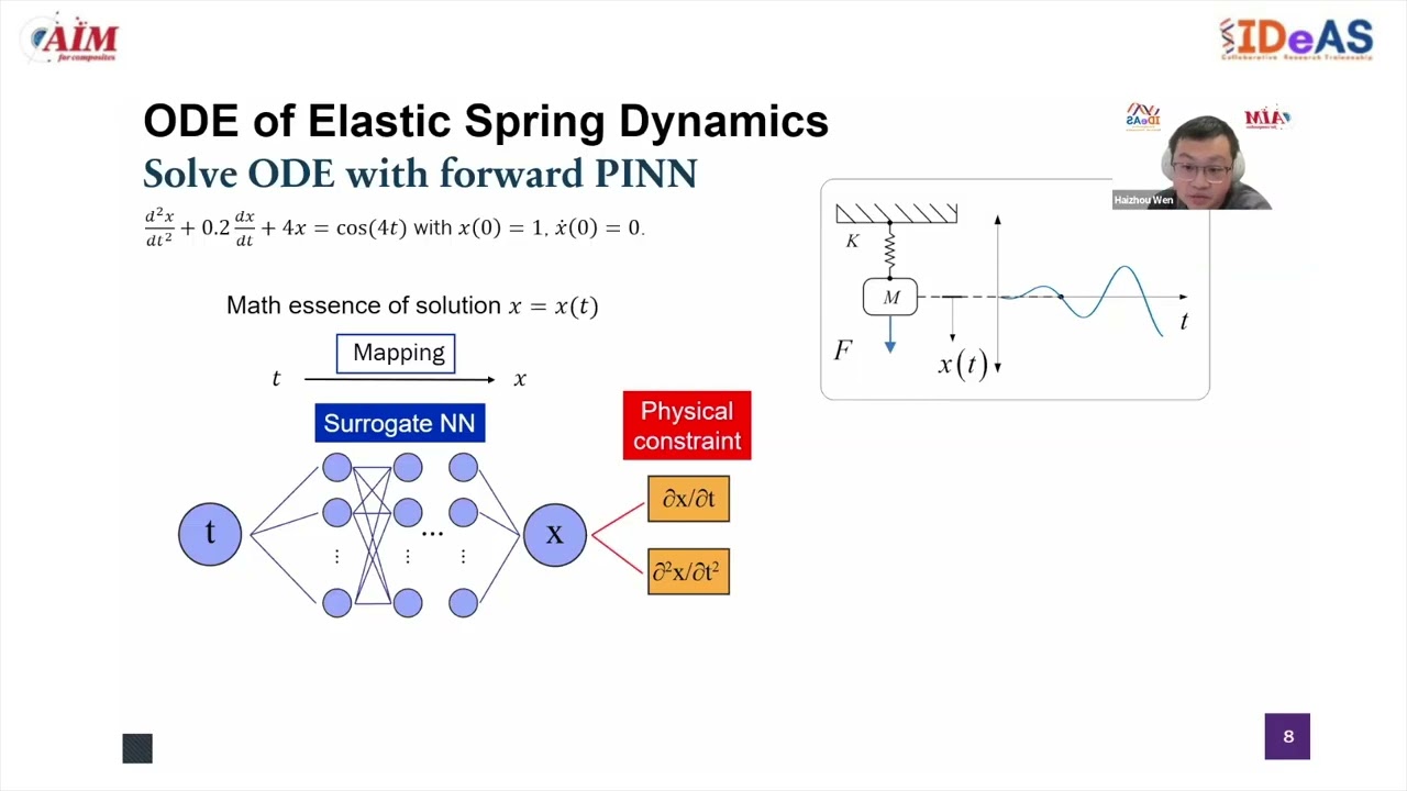


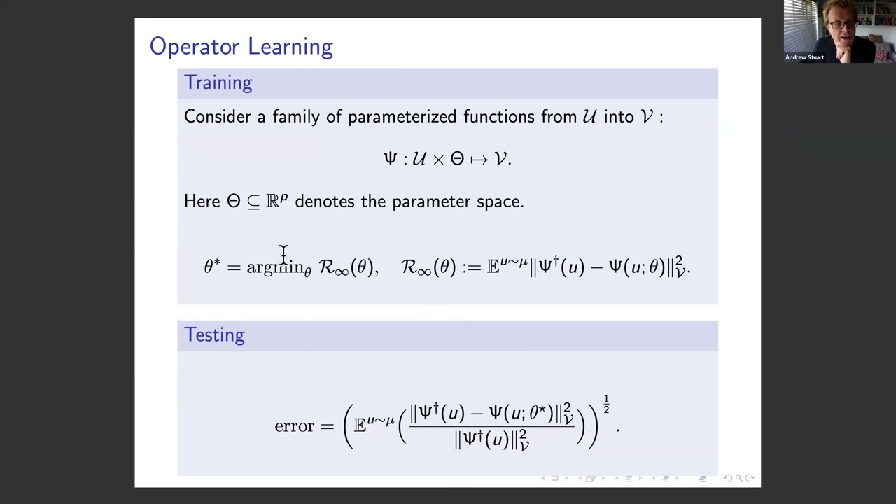


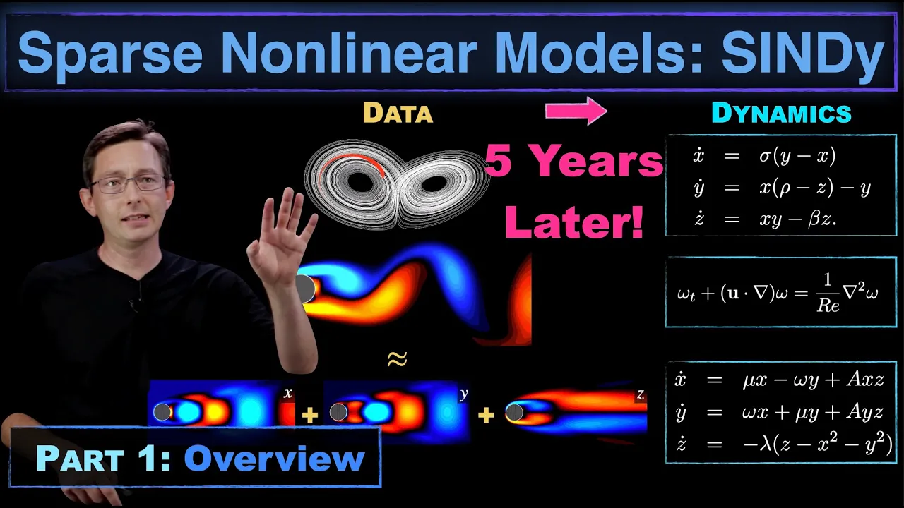

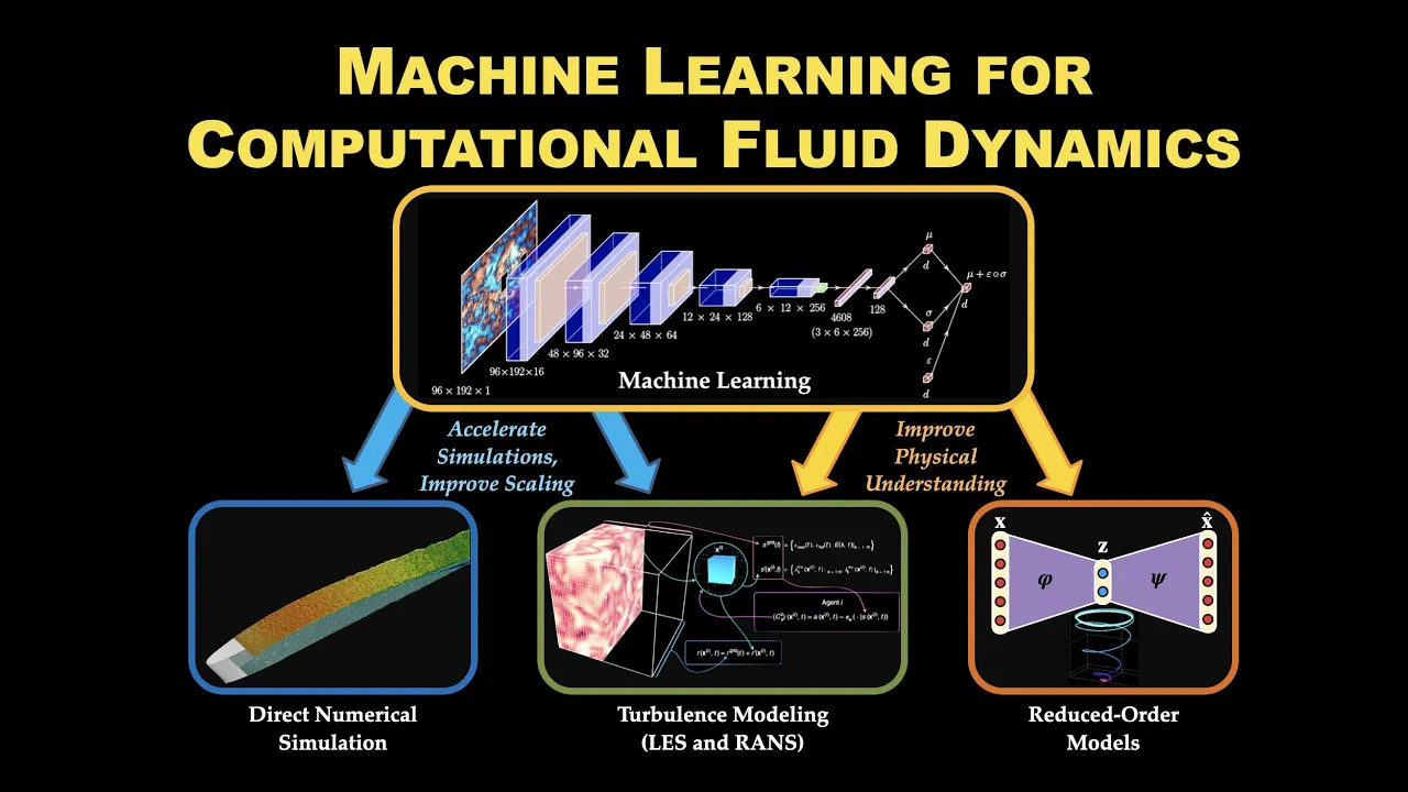



Physics-informed machine learning integrates physical laws directly into machine learning models by encoding differential equations into the model architecture or loss function, enabling data-efficient solutions to scientific computing problems such as solving partial differential equations, performing design optimization, and conducting inverse problems with minimal data requirements.
Hidden Physics Models: Machine Learning of Nonlinear PDEs
Added:Fundamental theory of Partial Differential Equations (PDEs) and classical numerical simulation methods, such as Finite Difference or Finite Element Methods.
Core concepts of Deep Learning, specifically multi-layer perceptrons, optimization algorithms (e.g., Adam), and backpropagation.
Automatic Differentiation (AD), which is the computational backbone for calculating exact derivatives of neural networks with respect to their inputs.
Basic understanding of inverse problems and parameter estimation in mathematical modeling.
In-depth study of Physics-Informed Neural Networks (PINNs) for solving forward and inverse problems in complex geometries.
Neural Operators, such as Fourier Neural Operators (FNO) and DeepONets, which learn mappings between infinite-dimensional function spaces.
Data-driven discovery of governing equations using sparse regression techniques like SINDy (Sparse Identification of Non-linear Dynamics).
Scientific Machine Learning (SciML) application areas, including turbulence modeling, climatology, and biophysics.
Uncertainty Quantification (UQ) in physics-informed machine learning to assess the reliability of model predictions under noisy data conditions.
20.4K views561likes50:06Original Release: 2019-11-12
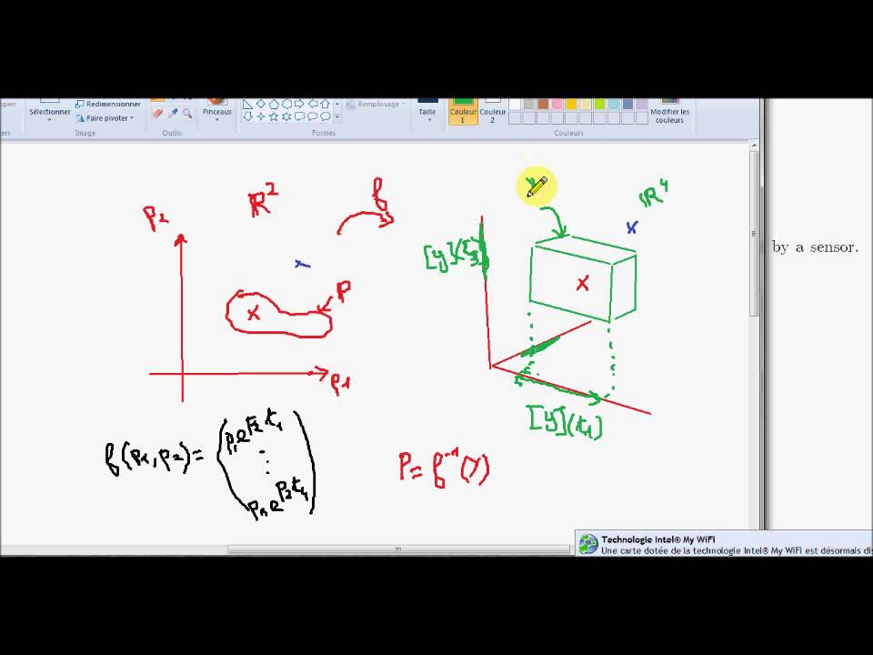
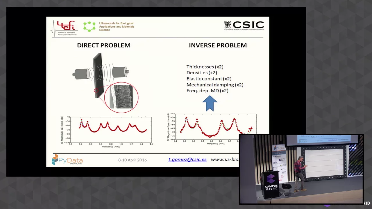
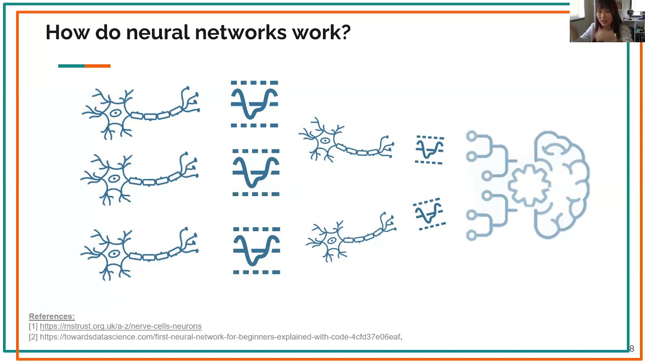
yes let's get it started my name is mozzie Ric research assistant and currently I video senior software engineer the guys above are not paying me anymore so I've been here for about 11 months now everything is started at Brown and I started with this project supported by DARPA and the project was design optimization of a super cavitating hydrofoil basically the problem is you want to go as fast as possible so that you create vapour around the hydrofoil and once you have vapor that vessel is basically flying in water there is going to be air around the hydrofoil and everything ended with this project where we have an aneurysm of a real patient and we are learning the dynamics basically the velocity and the pressure and the shear stresses on the wall of the aneurysm given data that are coming from CT scan or 4d MRIs a spacetime MRIs I will go through basically the historical account of how things developed and where we are now I'm not going to be talking about these three topics I'm not going to be talking about classification translation or learning a high dimensional probability distribution on this space of images but there is a message here the data dictates the model if you have images and your task is a classification task then probably a convolutional neural network that has a sparse structure is a proper tool if you have a language task probably a sequential model like a recurrent neural network or lsdm and these days even convolutional neural networks might work for it if you have if you lack data that are labeled you have unlabeled data you can work with unlabeled data learn the probability distribution and generate images that look like reality in scientific computing we lack data that's our problem for instance for designing that super cavitating hydrofoil we don't have data the data is going to be building that pink the vessel putting it in water testing it multiple rounds that's not possible the alternative is doing simulations and this is what we did we were using simulation but simulations are expensive because these are navier-stokes equations we have to do turbulence modeling and there are expensive models they take around six hours each round of the data generation and basically labeling your data so at that time we thought this is a problem we want to do design optimization of a super cavitating hydrofoil that's the engineering look at it we today we do a 2d cross-section we get 17 or 18 parameters with you our simulations and we get lift over drag now this is a function from a high dimensional space to a low dimensional space we can put a surrogate here for our solver basically and we are looking for data efficiency this is key data efficiency is a key concept today we are started with Gaussian processes because they are data efficient for a Gaussian process the input is one of those high dimensional shapes X I and Y is the lift over drag that's going to be our data coming out of simulations pairs of X I Y I and we are going to be doing regression with data we are gonna write a model for the data and that's our model we have annoys model that's normally distributed if you write it in vector form you get Y is equal to f of X plus Epsilon now epsilon is high dimensional it's basically your data for prior we say we are gonna put a Gaussian process there what is a Gaussian process it's just a shorthand notation for this concept basically you take any two points of that function evaluate it you get f of X f of X prime those two points are correlated they are normally distributed and the distribution is given by this rather than writing this all the time we are gonna say f of X has mean 0 and this covariance function the assumption is that if you have two points that are very far apart from each other probably they are not affecting each other that much this could be one assumption and those assumptions you can put them here in your kernel that's exactly what I said right now this is the covariance kernel that's going to do that for us if two points are very far from each other this exponential with the negative sign is going to make that go to zero therefore they are not that much correlated you can have multiple different kernels but that's gonna be the choice of your prior this is a choice that you have to make this is a choice that we had to make this assumption once you make those assumptions everything is normal the data assumption was normal cow geometry is normal therefore you can say my data is normally distributed with mean 0 and the covariance matrix this time we are evaluating the covariance kernel at those points and we are adding the noise now we have a likelihood and once you have a likely that's nice because you can do maximum likelihood or you can do minimize the negative of the log of the likelihood that's coming out of the normal distribution normal distribution has an exponential term the log is going to cancel that out and that's the term you get why do we do that because we want to find the best kernel among all the cameras that we assumed that's the purpose of training once the training is done we have to do prediction or do inference somebody gives us a new point X star and tells us what is the value of that function at this point based on our assumptions and the data assumption we can write down the correlation between that new point and the data once you have that we can condition on the data you get a mean you get a variance that's the mean and this is the variance so the beauty of Gaussian processes is that there are data efficient why because they are balancing the trade-off between date of it and model complexity during training time once the training is done we get a nice uncertainty bound around our predictions so that's another advantage we can do uncertainty quantification let's go back to our example where we were trying to do design optimization this is their space the design space in our case it was 17 or 18 dimensional I'm projecting everything into a one dimension and on the y-axis we had our simulations the blue curve if we had it that would be a luxury because we knew what is the lift and drag for every possible scenario that could have but we don't have it the blue curve we don't have this function the blue one we see it through observation through data which could be noisy these are our simulations given this geometry what is the lift over drag given that other geometry what is lift over drag we do a regression using Gaussian processes and we get that basically Gaussian processes I want you to think of them as function approximator z' during this talk don't think of them as distributions they are just function approximator x' and if we go back to this slide probably I shouldn't do it this is just a linear combination of our kernel if we expand if we call this alpha it's going to be alpha times the kernel similar to the RBF yes equivalent to what so probably it's very close it's equivalent to SPD's yeah exactly it's basically RBF also you can think of them as RBF Karen Olsen yeah this is equivalent but usually this step is ignored that's the contribution of machine learning among all of the possible basis functions give me the best one this round of this is a very important round the training ground so how do we use the uncertainty we are store with two simulations one is here one is here we do a regression the blue key remember we don't know it and that's a very bad prediction of the underlying function what the uncertainty is telling us something if we take the mean plus to a standard deviation of the uncertainty that's going to give us a it's not the best one an acquisition function now this guy we can optimize we can query what is your maximum and it's kind of tell us your maximum is here we go ahead and sample at this point we add another data we run our simulation once the function change is the acquisition function is going to tell us go sample here we are going to go sample there the prediction is getting better we are trying to find a maximum of the blue function through observations and we already we are already very close we had four observations one two three four we keep doing that in the next round the algorithm is thinking maybe the maximum is somewhere else maybe the maximum is here because there is huge uncertainty in the prediction that step is called exploration so we explore explore again explore again exploit so we are balancing the trade-off between exploration and exploitation for those of you who know the multi-armed bandit problem this is close to that explore exploit explore exploit exploit and we found the maximum and that and we didn't need to run our simulations in this part of the domain now if your underlying dimension is huge this is really beneficial we want to go even one step further we want to become even more data efficient we had two simulators one was Reynolds average navier-stokes solver which takes six hours for each simulation and we add a potential flows over which takes four minutes can we somehow use that data the low fidelity data is cheaper to obtain but it's less accurate we are going to write a model we say too high for that this is an assumption this is a prior assumption that we have to make we make a prior assumption that the high fidelity is a low combinate is a linear combination of the low fidelity plus some noise plus some correction and both of them are gaussian processes this guy on that guy and I'm gonna do this exercise we are going to keep adding data on the low fidelity basically running the cheaper solver without adding any data to the right side and we keep adding data there and I want you to focus on their right side so the low fidelity data along with Gaussian processes along with some neural networks helped us improve the already optimized design using genetic algorithm that one is optimized using genetic algorithm and we optimized it even further there is no physics here everything is data driven so far we are being data efficient we are doing our best but when we are solving that problem the reason of your Stokes there is physics can we somehow encode that physics inside the kernels that was the question can we somehow physics inform our carenotes so the difference here is now you have two functions low-fidelity function high fidelity function and they are correlated any point on this function is going to affect a point on the other function and we are leveraging that by conditioning on the already available data that you have on the low fidelity what's that good camera physics inform let's say this is our physics burgers equation UT + uu x a coefficient u XS is equal to 0 we discretize backward euler u n minus u n minus 1 divided by delta T is the right hand side we approximate u n by a Gaussian process so here's the question why am i approximating u n by a Gaussian process why not u n minus 1 we had a choice to make put the prior here on you add or put a prior on U n minus 1 if you put it on UN minus 1 you have to solve a PDE you have to integrate a partial differential equation but if you put it on UN we can take derivatives and taking derivatives is easier and the whole talk of today is about derivatives and we as human not knowing that we are really good at taking derivatives but we are so let's leverage that here we are going to take derivatives and do symbolic derivatives mathematical maple nothing fancy we can write down the correlation between UN and un minus 1 this is the kernel that we started with this is K this is K and n minus 1 and look at the four compare it to the equation our equation is inside the kernel okay plus delta-t UN minus 1 K X coefficient K X X so this is cool now any sample that you generate at random from this distribution is going to satisfy this count this equation by construction so how do we take the physics out we take the physics out using data our data is our initial condition everything is data the initial condition is a data but we don't see the blue curve we see the red dots some of them are really outliers given this data and boundary condition we are gonna train the hyper parameters of this Gaussian process and the training is done using maximum likelihood basically we are finding the best basis function among all those possible best prior you find the best prior then we do prediction into the future by conditioning on the data you condition on the data you do prediction that's one step from time 0 to time delta T so how do we continue from time delta T 2 to delta T should I take the kernel and do the derivation again make more derivatives out of the kernels which really costly so we are going to summarize the information inside the data what do I mean out of the posterior here we're going to generate artificial data at some random locations we can evaluate that function anywhere we want they mean we are going to use it to do prediction and do training there is a variance here that we have to propagate that's the only trick from time delta T 2 to delta T and we keep doing that we solve burgers equation we get the shot and we get a nice on certainty bandwidth around the solution any of these samples from this distribution could be a solution to the burgers equation so we are quantifying the uncertainty the method is sort of honest it's tell does any of these samples could be your solution I'm not sure which one the other day I wrote down the math and compared on one tape on one board Calma filter which is a finite-dimensional for Odie's this one is for infinite dimensional PDE s so we are not discretizing the space there is one-to-one correspondence between the math and comma filters are important they took us to moon this is happening in infinite dimensions that was for a forward solver basically I give you initial and boundary conditions give me the solution now can we do inverse problem if I give you data even inside the domain can you tell me what are the parameters of the PD that's an inverse problem now we have more data and we have more unknown let's go through the math real quick we discretize with a Gaussian process on un push it through the differential equation that's the physics in form prior so nothing changed except for one thing the parameters of the differential equation lambda 1 lambda 2 lambda 3 turn into hyper parameters of this kernel the same maximum-likelihood methodology that we used to do training and find the best Thetas we are going to use the same methodology and find what is lambda 1 lambda 2 and lambda 3 so the cost of this is the cost of a forward solve and you do inverse it's very data efficient for two reasons one is that Gaussian processes are data efficient we have nothing to do with it the other one is this is a physics inform prior we are putting a lot of structure on this prior that's why given the chaotic dynamics of coromoto Sowinski equation we can use only two snapshots in time that are delta t apart and find out what are the parameters even in the presence of noise chaotic system very little data and noise being added chaotic system very data very little data with noise and that's the noise on the data that's basically the data that we are using you can do now your stocks flow past a cylinder to it snapshots of this one not the whole time series not the entire spatial temporal time series two snapshots and we are learning their coefficients in front of them basically what is the Reynolds number and the Reynolds number corresponds to the shape of the object in front of us like what is the size of the object given the flow pattern behind the cylinder and that's basically a real experiment that we try to do and we failed this is real data we failed not because the method cannot do it but because the data had gravity inside it and we were not modeling gravity at the time so far Gaussian processes a machine learning framework is helping us do scientific computing can we help Gaussian processes back Gaussian processes are not scalable to Big Data because you have to invert that covariance matrix it's a full covariance matrix if you have that's the size of data cubed that's the cost of it the idea is okay you have this big data set maybe most of this data is redundant can you do data reduction what if you have millions of data what if 10 of them are just important or informative it's similar to high dimensional not all high dimensions being important but some of them being important at low dimensional manifold maybe not all of the data is important some of them are more important than others can we find those and the idea is coming from the ocean processes itself the ocean processes has this prior gives you the posterior now the idea is the posterior could be your nuker not your new prior condition and that get a new posterior that your new prior and keep doing that but keep conditioning on mini-batches of date and keep updating these red circles basically we are summarizing this big data set into 8 hypothetical data set and this idea is coming out of numerical Gaussian processes where we had to generate artificial data out of our posterior the same idea and it's an idea that makes sense this is how human think we start with a prior uninformative prior then some data comes in we condition on the data we update our prior then some other observations come in we update our prior about the world that's what's happening here where did we apply it this is Cape Cod area near Boston and we applied it on satellite images and satellite images are spatial temporal data sets and what are we measuring this is the sea surface temperature some days are cloudy so you have very few observations some days are sunny you have a lot of observations some days are partly cloudy and whenever you have a spatial temporal time series that's huge data that's big data so a Gaussian process cannot do it we have to summarize the data and we summarize the data setting to 1000 data points and that was enough to give us a mean prediction and uncertainty prediction and the uncertainty is nice it makes sense it's going down here where we had some data so the first part is over I hope I didn't tire you the next one is about neural networks can we do the same thing using neural networks can we physics in for neural networks for Gaussian processes we were using symbolic differentiation basically mathematical maple there the only reason I mean one of the major reasons neural networks are successful is because of automatic differentiation so we are good at taking derivatives we as human let's leverage that one let's start with the concept of regression it's similar to before the data is the same as before this one is familiar if you have a function you can write it as a linear combination of some basis this is what we do in scientific computing all the time we write bases but what if you can't learn the bases without this guy it's going to be boring our basis is a linear combination of another basis then it's going to be linear everything is linear it's going to be boring we put a non-linearity here to introduce non-linearity it doesn't have to be tonnage it could be rail u it could be switch activation function you name it we can get creative then what is H L minus 1 a linear combination of another set of basis functions that I thought H 1 is a non-linearity applied on a linear combination of another of the input actually for Gaussian processes everything was about the covariance for neural networks everything is about the mean that's coming out of our noise assumption that's our noise model that's our likelihood model now we can write down our likelihood that's the likelihood that's another form of the likelihood basically it's just mean squared error so mean squared error is sort of like likelihood where you ignore the noise when you don't optimize over the noise prediction do you remember for Gaussian processes was tough we had to condition on the data we had to carry the data with us all the time with neural networks we are summarizing the data in these parameters the airport prediction is easy once you train the parameters and it's fast and it's efficient Gaussian processes versus neural networks Gaussian processes are nonparametric what do I mean you have to carry your data with you all the time you have to condition on the data the wrong networks are parametric and these are the parameters Gaussian processes do not scale to big data because you have to invert that matrix neuron networks are scalable why because you don't have to do your summation over all of your data we can do mini batching to get an approximation of your gradients to do training Gaussian processes quantify uncertainty neural networks don't the ocean processes balance the trade-off between data fit and model complexity neural networks no role networks can over fit unless you do regularization of different kinds so these are the two extremes of this story you can mitigate the differences like scale Gaussian processes to big data set we saw an example but you have to work harder it's against their nature you can encode uncertainty into neural networks like dropout but you have to work harder let's physics in for neural networks we are going to approximate our function we don't you run Network it has a bunch of weights and biases and we use automatic differentiation to take derivative with respect to time X X X and you get your residual so our contribution is not coming up with automatic differentiation it has been around for a while our contribution is the way we are using it to obtain a neural network that knows about the physics that knows the equation this neural network F has the same parameters as neural network you same weights and biases and we do training this way Paris went through a nice way of doing the training better but this is the benchmark let's go with that this is pins and we can solve P DS that's one angle we can solve P DS but we know better ways of solving P DS like find a different thing is a very good one finite elements has been around for half a century spectral elements that's very efficient finite volume in the industry they are using it all the time and it's fast efficient okay we can solve PD is using neural networks that cool the other angle is that we can train a neural network using 100 data sets this is data efficiency from the machine learning perspective because we are regular rising our neural networks heavily with the physics that's the more exciting story that I like making neural networks data efficient it's coming on that's a very good question the question is about high dimensional PDS but let's go through the cost of physics in forming around networks what is the cost this is shown in your equation nothing special about Schrodinger's equation it has a real part in as an imaginary part so we are gonna put a neuron Network here up until this part this is physics uninformed the most boring possible type of neural network fully connected ten layers deep let's say 50 layers 50 neurons let's look at 10 layers we are gonna go and apply automatic differentiation once we take the derivative of this guy with respect to time and we are going to do back propagation when you do back propagation you're literally copying the adjoint of this guy and putting it here so we just doubled the length of the network we go and take the derivative twice we just double the length of the already doubled network another time so it's going to become 40 that's the cost you create a computational graph it's going to be a huge computational graph and it's going to be very deep so these are really deep networks these operations are non-trivial operations and now you write angular residual up until this point we are not committing any errors it's much imprecision accurate whatever we did your machine precision could be float32 10 to the power negative 7 but we committed no errors up until this point where do we commit errors we commit errors here and this is what Paris was talking about this is very important properly waiting this is literally open for research it's open territory and you can solve shading your equation that's the absolute value of the solution so I get this question a lot what is the difference between how do you compare pins with finite elements finite volumes finite differences how do you compare it with reduced order models let's compare it line by line let's say you want to do finite elements you have an infinite dimensional space of your solution and we have to find a finite dimensional representation in that high dimensional space we are going to choose basis we neural networks we are gonna choose a bunch of whip pins we are going to choose a bunch of neural networks to represent this space we reduce order models we choose them smartly like based on previous examples based on previous time based on similar geometries which is the basis differential operators finite elements writes the weak form finite differences discretize it pins use automatic differentiation machine precision so we didn't touch our operator reduce order models similar as finite element finite volume water for solver we use a linear solver or we use a nonlinear solver or we use a iterative solvers here we are using gradient descent to do training this is an optimization now similar for reduced order models for evaluation we do interpolation we do inference we do interpolation that's how you can compare pins as a forward solver with the landscape so there are not efficient pins there is low compared to finite volume their slope because of the training procedure because we don't want to hide the training ground you can go to high dimensional you can solve high dimensional TVs you can do high dimensional hamilton-jacobi bellman equation you can do high dimensional black-scholes equations and this is where we start to gain that advantage with pins why is that we'd find a different thing if you have a one dimensional space we can put ten point in your grid in twos in two dimensions you do 10 squared 100 in three dimensions 10 cubed points 10 to the power 4 5 it's out of the possibilities that's the curse of dimensionality we neural networks we don't have to worry about the cares of dimensionality because our degrees of freedom is not tied to this space our degrees of freedom or something abstract the weights and biases this is a is an abstract concept and they appear you know in all places like if you have 100 assets what is the price of an option on this 100 assets 100 is their dimension of your problem this is where we start gaining advantages another place is when we do inverse problems let's say we are collecting data behind the cylinder and we want to learn the Reynolds number these two parameters lambda 1 lambda 2 are gonna be added to 10,000 other parameters of the neural network and we're gonna train them using mean squared error that's fine to be honest when we were writing this paper we were trying to find these parameters what is the Reynolds number and the algorithm gave us gave us that this is okay it gave us something more it gave us the pressure without even having a single data under pressure the pressure is popping out of the continuity equation through optimization it's coming out of the physics can we do real stuff with it and at that time we had this idea what if we inject particles in somebody's arteries we track those particles and get the pressure drop and diagnose whether somebody has a heart stenosis or no and the stenosis is like this whether the doctor has to do a surgery or no without opening the patient up but that's a very stupid idea it worked we got the pressure we got the pressure drop it's a very bad idea because you cannot inject particles in somebody's arteries that guy is gonna die but people do for the MRIs all the time they inject concentration in our arteries all the time to do imaging bolus dye they do it all the time they can use the oxygen level of our blood to do for the MRI this is when we started experimenting with concentration data this is a passive scalar is just being attracted by the flow it has no effect on the flow and we were able to get the velocity and the pressure where we had different peclet numbers peclet number is basically how diffusive is that dye that's being injected in our body that's cool can we get a little bit more to do so what's the problem here we had a neural network we had observations only on that part right so we had observations only on this guy so you cannot do a regression on it and get these guys out unless you enforce the physics and this is how he enforced the physics using automatic differentiation this is our hidden physics an ideas like Mark of hidden Markov models are coming into place but everything is infinite I mentioned the loss is boring there is room for improvement here that's a data that's literally the data is spatial-temporal time series and we are cutting the data here we are not enforcing boundary conditions and we with PDEs boundary conditions are important without boundary conditions you don't have a solution it's not your niche we are not enforcing initial conditions PD is without initial conditions are not solvable if you cut an artery from here what is the proper pressure boundary condition there are ad hoc models for it but nobody knows because you are cutting this part from the whole arterial system of a human body given that data you can learn what is the flow like and given the equations learn the trajectories and the pressure and the shear stress everything is in the paper you can do lewis structure fluid structure interactions get lift and drag forces and the damping and stiffness of the solid you can couple all these and PD es like particles the oil Aryan and Lagrangian framework and get the Lagrangian out you can do turbulence this is the PDF of the concentration from the PDF of the concentration we can learn the conditional diffusion and conditional diffusion is hard conditions tougher tough to get I'm not an expert in turbulence but Peyman is and once he saw these results he was really happy because it took him pages of rigorous mathematics like derivations to come up with a solution to this problem you can learn dynamical systems by putting a neuron Network on there and learning it using a loss function that coming out of this hoodie you can learn infinite dimensional dynamical systems we can learn 3ds basically you are collecting data from here to here you learn the dynamics you extrapolate something cool we can change your initial condition and let it solve it that's kdv equation and thank you [Applause]
Up Next
91:39
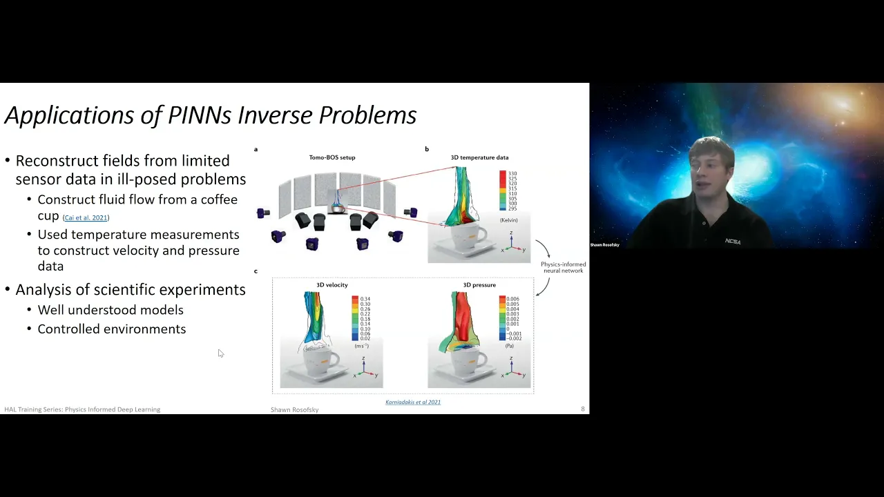
Physics-Informed Deep Learning: PINNs Tutorial (CAII HAL Training)
@NCSAatIllinois
2.1K views•2021-11-19
30:57
Solving PDEs/ODEs with Neural Networks | Physics-Informed ML Tutorial
@nptel-nociitm9240
57.7K views•2019-05-06

13:03
Bypassing Tor Censorship: Bridges and Pluggable Transport Guide
@Coding_ForEveryone
397 views•2024-06-11

18:41
Neural Networks Explained: Math, Layers, and Learning Fundamentals
@3blue1brown
21.9M views•2017-10-05
Related Study Plans & Knowledge Roadmaps
Structured learning paths in Artificial Intelligence
artificial-intelligence
PINNs: Fluid Dynamics with PyTorch & DeepXDE
01Calculus & Fluid Dynamics Foundations
02Deep Learning & PyTorch Basics
03Introduction to Physics-Informed Neural Networks (PINNs)
+ 3 more learning modules
32h6 modules
Explore Roadmap
artificial-intelligence
Aligning LLMs: DPO, TRL & Custom Datasets
01Foundations of Python & Machine Learning
02Transformers and Large Language Models (LLMs)
03Aligning LLMs: SFT and RLHF
+ 3 more learning modules
24h6 modules
Explore Roadmap
artificial-intelligence
Federated Learning: PyTorch, Flower & Privacy
01Python & Machine Learning Foundations
02Deep Learning Basics with PyTorch
03Introduction to Federated Learning
+ 2 more learning modules
35h5 modules
Explore Roadmap
artificial-intelligence
Securing LLMs: Guardrails AI & NeMo Gateway
01Introduction to LLMs, Python, and APIs
02Understanding LLM Vulnerabilities & Threats
03Defending LLMs with Guardrails AI
+ 2 more learning modules
15h5 modules
Explore Roadmap