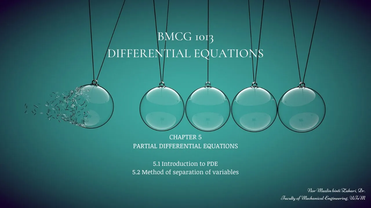
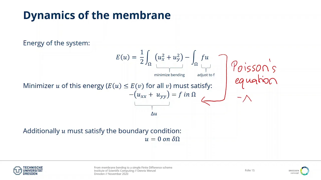
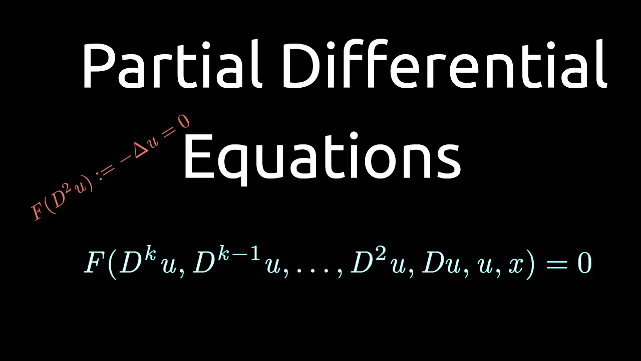
Partial Differential Equations: An Introduction to Canonical PDEs

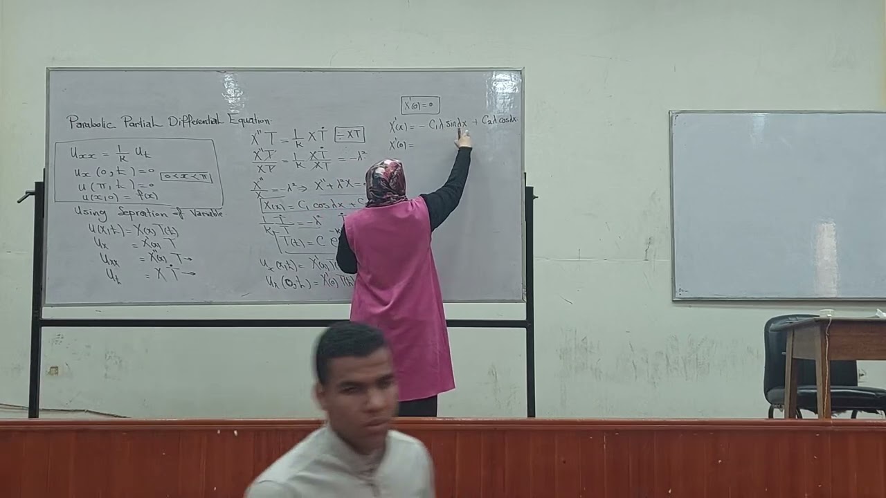
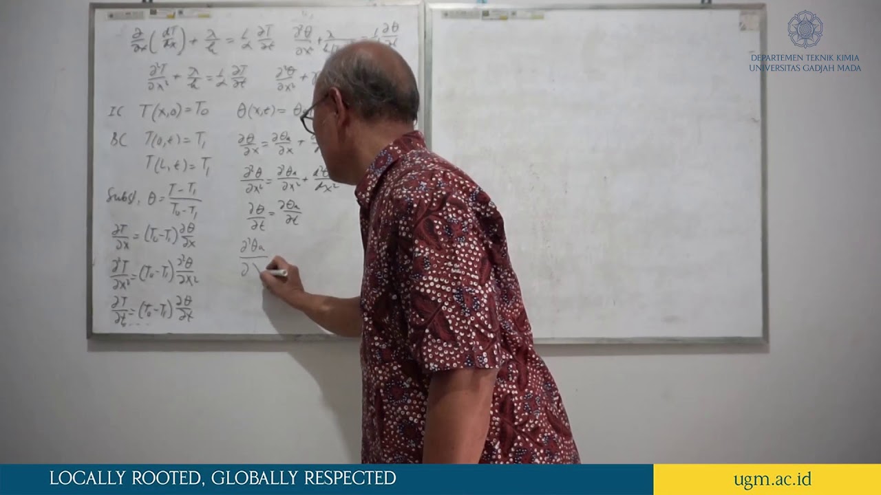
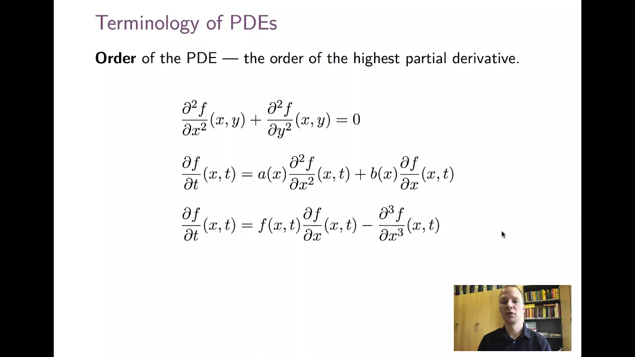
[00:00:09]welcome back so i am incredibly excited today  to tell you about partial differential equations and so in this video what i'm going to do  is essentially motivate what are partial differential equations why do we need to  solve them and i'm going to give you a lot of examples of types of pdes that come up  throughout physics and engineering and science okay so this is absolutely one of my favorite  topics um and i gotta say i am just so grateful to have the opportunity to teach  this to you it's something that has you know partial differential equations have changed my  life you know it allows you to solve problems that uh you can't solve without them and so i  really really hope that this is kind of opens a door to you like it did for me okay calculus is  kind of the same way it's one of those things that once you see the world through that lens you can't  unsee it okay so a partial differential equation there's a definition here it's essentially a set  of equations in terms of a multivariate function and its partial derivatives and  so the multivariate function um the multivariate function u  that i'm going to talk about u is often a function of space and time okay so this  is my function um x is space and t is time and this might be a this might be a scalar function  this might be the temperature distribution on this piece of glass here so x would be a two  dimensional x and y vector so in general this could be a vector u could be a vector and t could  be time or you could be a scalar like this could be the temperature distribution like i said this  could be the fluid flow vector field of the error in this room in which case you would have three  components the x velocity u the y velocity v and the z velocity w and x would be a  three-dimensional space vector x y and z so this is a very flexible function it's  a function of space and time typically and the partial differential equation  is going to relate this function and its partial derivatives so a good  example would be the wave equation so i could say the second partial derivative of u  with respect to time is equal to some constant uh some some positive constant times the second  partial derivative of u with respect to x so in this case u is a scalar function this is  just a scalar function and x is a scalar you know position along the x-axis and this would be  the equation for a wave uh you know kind of a wave u of x and t propagating at some constant  velocity c okay and i'm going to you know we can derive this we can analyze this this is just one  example of what a partial differential equation looks like so again it is a relationship between  some function u and its partial derivatives here i have a partial derivative and t and a partial  derivative and x now that's different than an ordinary differential equation so um you know if i  looked at my ode this is just a sidebar if i look at an ordinary differential equation it is usually  a single derivative of a function you know x of t equals some uh you know function of x like  lambda x of t and in this case there is only one variable that's being varied time so i have a an  independent variable time a dependent variable x and i'm just taking derivatives only with respect  to that independent variable time whereas for partial differential equations it has multivariate  dependencies it's a function of multiple variables x and time in this case or maybe even multiple  spatial dimensions and so i have to think about partial derivatives with respect to each of  those those independent variables okay good uh so that is just kind of an example or a  definition of what a pde is and this is an example what i want to do is i want to start building  up some of the most useful pdes that we use like all the time in physics and engineering and  science and then we're going to start thinking about what are some of those properties of those  pdes that are particularly useful so maybe one of the things i'll start with is i'll just kind  of describe some of the canonical canonical pdes and all of these canonical pdes that i'm  going to describe have some common properties so they are going to be linear and i'm going to  define what i mean in a minute so they're linear they are second order and they are what is known as homogeneous  or homogeneous depending on homogeneous okay so i'm going to define what each of these  means so linear just means that um the partial differential equation can be written in terms of  linear operators where there's no nonlinear terms like u squareds or u times u sub x and things  like that let me make a quick quick quick sidebar that oftentimes we use subscripts like u sub t  to denote partial u partial t and things like u sub x or u sub x x would equal the second partial  derivative of u with respect to x squared okay so often times partial derivatives are denoted by  subscripts and i'm going to do the same thing here so linear basically means that there are  no nonlinear terms there's no things like no no products or cross products no products  between my various u u sub x u sub x x terms so i don't have any u squareds or u times u x's  or u x times u x x's those would be non-linear and i'm going to talk actually about linear more  later so just to remember that second order means that there's no more than a second no derivatives  higher than second order no derivatives higher than second order okay so you know i could  technically have a fourth derivative and x a fourth order diffusion term there are physical  systems that have fourth order diffusion uh but at least in these canonical pdes i'm going  to write down here we're only going to think about second order pdes and uh homogeneous means that  there is no time forcing or spatial forcing so the the governing rules of the system are the same  throughout time and they're the same throughout space now for example in this wave equation this  is essentially the equation for a guitar string okay and you could imagine building a guitar  string where the first half of it is nylon and the second half of it is steel and in that  case that will be a non-homogeneous differential equation because the the rules of the equation  will change on those different halves of the guitar string because the material properties  will mean that the c is different in one part of space than in another part of space so  what homogeneous means is that there is no um time dependent forcing or spatial  dependent forcing no time dependent forcing or space dependent forcing and you know now that i'm thinking about  it that example i gave you is actually not a good example of an inhomogeneous equation  so i can have an equation where the constants themselves are functions of space um you know that  that's okay but i guess uh here what i mean is if i actually actively force my system in time or in  space if i have some plus forcing function that's a forcing of time and space and i'll give you lots  of equations examples of this for example in the heat equation if i have a blow torch and i'm you  know actively heating up a metal plate that would be an inhomogeneous term in that equation so we'll  we'll talk through all of this in a minute but these are the three kind of basic properties for  these canonical pdes i'm going to write down now and so i want to write down three basic  partial differential equations we have we have the wave equation which i've actually already  written down before we have the heat equation this is one of the most  important equations in all of physics the heat equation and we've already seen before when  we looked at potential flow we have laplace's equation laplace's equation and laplace's equation  and heat equation are very very closely related so here what i'm going to do is i'm actually going  to write these down and then we're going to talk about what their properties are we're going  to confirm that they're linear second order homogeneous equations so the first thing i'm  going to do is i'm going to write it down in kind of a specific form for two independent  variables so the wave equation is u sub t t equals a positive constant c squared u sub  x x that's actually exactly what i wrote down here just using subscript notation and this is  for a one dimensional wave equation i have two independent variables i have time and one spatial  coordinate x okay so this is a 2d version the heat equation is another super important equation so  this one again for for a simple case is u sub t a single time derivative a single time derivative of  u equals another positive constant we're going to call this alpha squared times u sub x x now these  look extremely close to each other all that not i pluck it you know i available these these  standing waves or if i take a a rope and i whip the rope it will send this traveling wave  traveling along that rope and the shape will kind of remain constant whereas for the heat  equation if i have some temperature distribution in a one-dimensional piece of metal immediately  it's going to start to diffuse and average out until it all becomes a constant temperature  which is very very very different behavior just because of the single additional  partial derivative in this wave equation okay and the the third canonical pde that we  always study uh in physics is laplace's equation which is just the heat equation if i set u t equal  to zero it's the steady state heat distribution uh like let's say i have a metal plate and i  heat one side you know in a hot bath and one side in a cold bath and i insulate the other two  sides there will be a steady state temperature distribution that is given by laplace's equation  so again i'm going to write this in two dimensions as u sub x x plus u sub y y equals zero  now notice i'm actually writing this in two dimensions this has two so so there's no time in  laplace's equation because it's for steady state heat distribution and so this would be  how the the steady state heat distribution has to satisfy this for a two-dimensional uh  heated object for example with boundary conditions and again we already saw that you know we  already saw this from the potential flow equations also solutions of laplace's equation  are potentials that we can use for potential flows good so these are three canonical pd's i also  want to show you what this looks like in vector calculus notation for arbitrary dimensions because  i think you know we've been essentially building up partial differential equations like laplace's  equation using vector calculus div grad and curl and so i want to show you what this looks like  for those cases as well okay good um so the wave equation in nd is going to look like u uh u sub  t t equals again some positive constant now times the laplacian of u okay and uh this is going to be  so if u is a function of x y and z this is now you know second partial of u with respect to x squared  plus second partial of u with respect to y squared plus second partial of u with respect to z squared  and you could in fact write down an n dimensional a 10 dimensional laplacian operator if you like  it's easy same thing for the heat equation it's just u sub t equals a positive constant alpha  squared again times the laplacian operator of u and laplace's equation aptly named is just  the laplacian operator of u del squared u set equal to zero and so these are kind of  the n dimensional this this would give you the steady state heat distribution not just in a  two-dimensional plate but in a three-dimensional object then you take the three-dimensional  laplacian or an n-dimensional object sometimes for example in machine learning you might  add some kind of artificial diffusion on an n-dimensional vector and you would need to be  looking at an n-dimensional laplace's equation now there are more complicated pdes that  we use in our daily lives like the navy or stokes equations are non-linear equations  okay so they are they don't satisfy this kind of nice property that the solutions uh satisfy  superposition there's other equations that are you know not second order like i  mentioned that if you had u quadruple x there are systems that have that kind of  fourth order diffusion i can have systems that are inhomogeneous i'm forcing them in space  or in time okay actively forcing those systems and so we can essentially relax all of these but These are the canonical building block partial differential equations that we use to build intuition to understand solution techniques and so we'll actually spend a lot of time thinking  about how do you solve Laplace's equation in fact we can derive separation of variables  one of the most powerful techniques to solve PDEs we can demonstrate it on Laplace's equation  and then use it to solve the heat equation you can use the Fourier transform techniques to  solve the wave equation and so these all become very very useful as building blocks to  understand how partial differential equations work good... are there other things I want to tell you?  I'm sure there are... in fact I think I'm going to tell you lots more in other videos maybe one  of the things I'll mention is what does it mean to be a linear PDE. So we've talked a lot about  this for ordinary differential equations. We know that we like linear ordinary differential  equations specifically because it means that linear superposition holds. If I have two solutions  of a linear differential equation, and I add up that solution, it is still a solution. And that  also is what linear means for PDEs. So let me just write this out... so linear is just a way  of saying that superposition holds and so what that means... let's take the wave  equation, for example, if I have two solutions of the wave equation I have two waves that are  traveling at some constant speed, I've got two solutions u1 and u2 and I add that solution  up... I superimpose that solution, it will also be the solution of the wave equation, because  this is a linear partial differential equation.

[00:16:28]And in fact, like I mentioned, all three of these  equations are linear. That is super super useful.

[00:16:34]So Laplace's equation tells me what the gravitational potential or the electric potential is going to be in a medium  away from charge densities or point masses.

[00:16:45]And again because linear superposition holds I  can have 10 charges and just add up the fields from all of those charges to figure out what the  field is going to be at some distant location x Linear superposition is one of the most  powerful tools we have in all of mathematics to handle differential equations. I'm going to  say it again: When we say superposition holds, this means if u1 and u2 are solutions to the PDE, then in fact any constant alpha*u1 + beta*u2  is also a solution. And so that allows us to essentially cook up basis solutions or "eigen"  solutions and then take linear combinations of those for more complicated problems, for more  complicated boundary conditions, geometries, etc., etc. And, in fact, that's how Fourier  analysis was invented... Fourier himself invented this Fourier transform specifically to provide a  basis of eigen solutions for the heat equation.

[00:17:59]So the heat equation, you can essentially  transform this into some diagonalized system using these sines and cosines... this Fourier  transform that Fourier invented, and it simplifies the heat equation and it provides  a family of unique orthogonal basis solutions, so that any combination of them also satisfies  the heat equation. Really, really powerful stuff. So we'll talk about all of this more, but I  really, really just love this idea that linearity allows you to add up independent solutions of  these equations and there's still a solution.

[00:18:35]And linearity also relates to the operators  themselves. So remember we're talking about this Laplacian operator, del squared is equal to the divergence of the gradient of whatever  function... so if I have the laplacian of "f" it is equal to the divergence of the gradient  of "f" for some scalar value to "f" and essentially these the gradient and the divergence  operator and therefore the laplacian operator are linear operators the partial derivative  of a function u is a linear operator on u and so that's something i really want to to  convey to you this is a kind of an abstract concept but very important is that i'm just going  to give you some examples of linear operators so a linear operator on u one example would  be if i just multiply it by a constant if i take u times 5u that's a linear operator and  you can verify this because you can plug in u1 plus u2 and that's still equal to 5u1 plus 5u2  it's the linear operator of u1 plus the linear operator of u2 so it's linear another linear  operator and this is really important and i want you to verify this this is extremely important  is the partial derivative of u with respect to x in fact the partial derivative of u with respect  to any of its uh the variables it depends on partial u partial t partial u partial x  second derivative of u with respect to x the laplacian of u the gradient the  divergence you know all of these are linear operators and so i want you to actually  verify that uh this l of you know alpha u1 plus beta u2 right so if if u1 and u2  are solutions then i want you to plug in this and confirm that this is alpha times  the operator of u1 plus beta times the operator okay this thing is kind of a pain to  erase uh plus beta times the operator of u2 and i'm just going to say this again so what  linearity means is that if u1 and u2 are solutions to the pde then alpha u1 plus beta u2 is also a  solution and what that means for a linear operator we build up this pde using these linear operators  this is a linear operator on u this is a linear operator on you multiplying by c squared is a  linear operator on u this is all kind of l of u equals zero a linear operator of u equals another  linear operator of u and so to confirm that an operator like a partial derivative is in fact  linear we verify that if we take two functions u1 and u2 and we add them up in some combination  a plus b then we hit that with the operator you can essentially you know pop the operator  out you can pop these constants out and you can split the sum so that it is equal to that  constant a times the linear operator of u1 plus that constant beta times the linear operator  of u2 and i'm gonna have you like get a piece of paper actually verify this is true for partial u  partial x verify it's true for second derivative of u with respect to x or for the laplacian  of u with respect to a multivariate function of let's say x and y really really really  important okay and these are all linear pdes maybe the last thing i want to show you before  you know we'll talk more about pdes a lot in the next few lectures so i don't want to overload you  here but maybe what i will do for the last thing is just give you an example of a non-linear  so this is not going to be a canonical pde it's a non-linear pde and this non-linear pde is  going to be berger's equation so burgers burgers equation it sounds delicious i'm quite  hungry so this is kind of a non-linear burgers equation and i'm just going to write out  what this pde is and then we'll talk about why it's non-linear okay so the partial differential  equation for burgers equation in one component is the time derivative u sub t plus u u x equals  some viscosity uh u x x so again this is for the one-dimensional burgers equation this u is just  a function of time and a single spatial variable x and it also is going to be describing how waves  propagate uh in space and time but because we have this non-linear term here this is a product  this is a product of u and u x this is not linear you can try to do this for u u x and this  is not true so that's another thing i'd really like you to verify that this is non-linear  and it's called a nonlinear uh convection okay that's a really important term here and  we'll talk about burger's equation and the physics more later but i also want  to point out in vector form you can write this as a vector u sub t this is for  a higher dimensional burgers equation plus u dot grad of u plus my sorry equals i i have  to erase twice in one video okay good this equals my laplacian operator my new times laplacian of u and i'm going to say  that this is for a vector valued u so now u could be the velocity in the x  and the y component so this u could be u equals you know u in the x direction and v in  the y direction and it's a function of x and y and t so now i have to use these partial these kind  of gradient and laplacian operators to account for those those partial derivatives okay good so  let's just take a step back and do a quick summary uh to wrap up so partial differential equations  like ordinary differential equations like calculus is one of the most powerful tools we have to  describe systems that change in space and time the world around us changes in space and time  so your brain has you know it's changing as a function of x and t constantly the atmosphere  the climate is changing as a function of space and time the ocean is moving and flowing  as a space function of space and time and this partial differential equation framework  allows us to relate that function we care about and how it changes in space and time through these  relationships of partial derivatives generally speaking we want to solve for this unknown  function u we want to solve this equation for u that's usually the goal and that is typically  easier to do for these linear pdes because if we can solve for kind of a basis of solutions  then linear combinations of those solutions also are solutions uh but there's a lot of interesting  equations like this burgers equation is basically uh kind of a 1d analog of the navy or stokes  equations and so you know for really nonlinear fluid flows it you're not going to have that  linear superposition and we're going to have to have other other solution techniques okay a  lot more on this coming soon stay tuned thank you