
















![[한화에어로스페이스 고명석 박사] Physics-informed Neural Network-based Virtual Sensors](https://i.ytimg.com/vi/OycWHAw_hTg/maxresdefault.jpg)



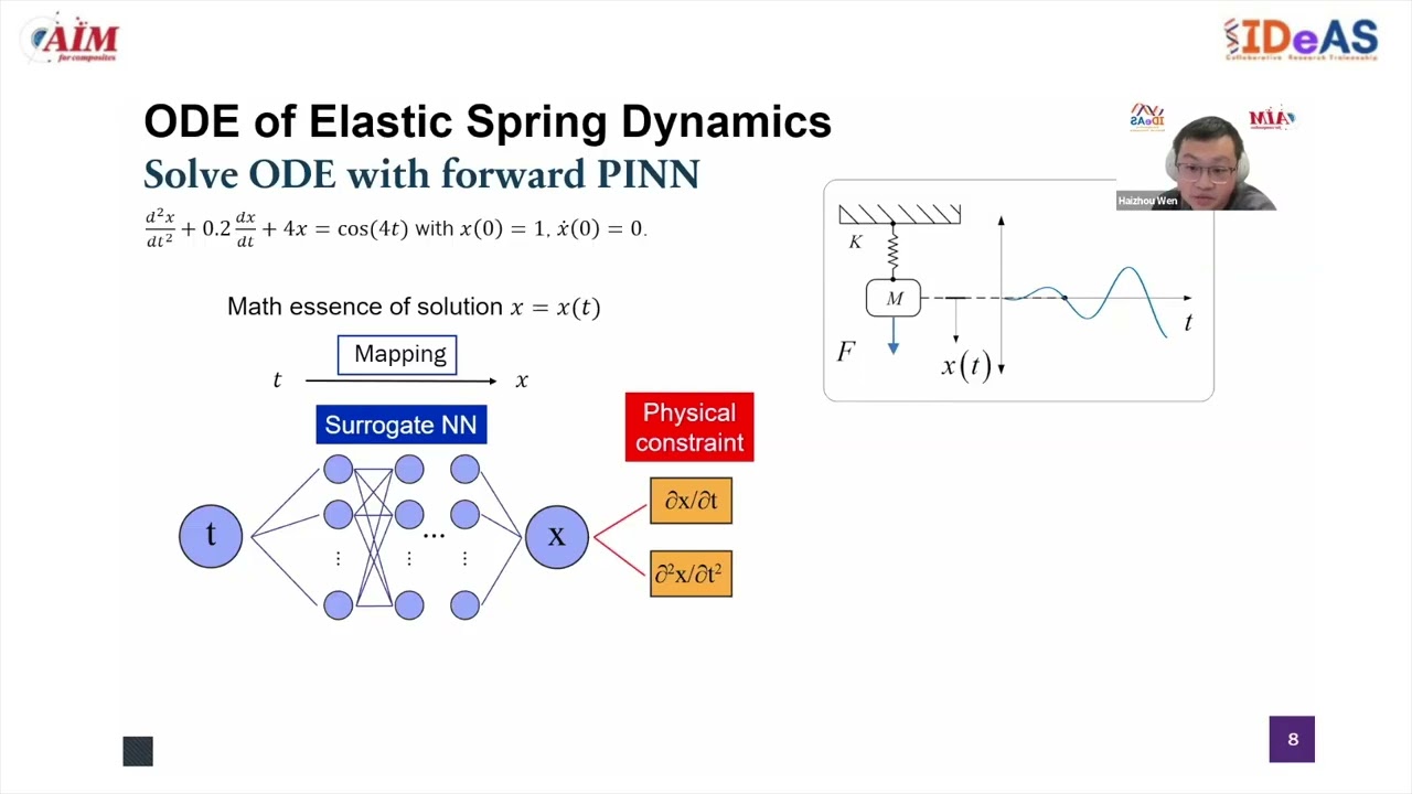
Physics-Informed Neural Networks (PINNs) solve differential equations by incorporating governing physical laws directly into neural network training, using the differential equation itself as an infinite source of training data rather than traditional datasets; the neural network minimizes the residual error of the governing equation while satisfying boundary conditions, enabling solutions to complex boundary value problems without requiring extensive experimental data.
Solving 1D Poisson Equation with Physics-Informed Neural Networks
Added:Fundamentals of Ordinary and Partial Differential Equations (ODEs/PDEs), specifically the mathematical formulation and physical meaning of the Poisson equation.
Basic concepts of Deep Learning and Neural Networks, including multi-layer perceptrons (MLPs), activation functions, and the backpropagation algorithm.
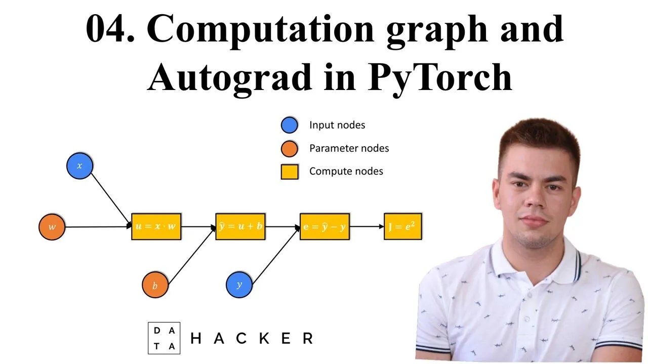
The concept of Automatic Differentiation (Autograd), which is crucial for computing derivatives of neural network outputs with respect to input coordinates.
Core optimization methods used in machine learning, such as Gradient Descent, Adam, or L-BFGS optimizers.
Familiarity with scientific computing in Python, particularly using deep learning libraries like PyTorch or TensorFlow.
Scaling PINNs to solve higher-dimensional PDEs (such as 2D/3D Poisson, Heat, or Wave equations) and handling complex domain geometries.
Solving inverse problems and parameter estimation, where PINNs are used to discover unknown physical coefficients from observational data.
Advanced PINN architectures and optimization techniques, such as Self-Adaptive PINNs, Gradient Pathology mitigation, or DeepONets (Operator Learning).
Applying PINNs to complex non-linear PDEs, such as the Burgers' equation or the Navier-Stokes equations for fluid dynamics.
26.9K views795likes16:44Original Release: 2024-08-08
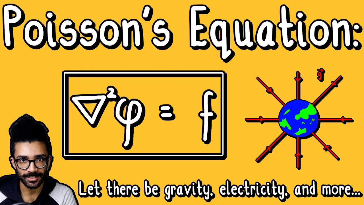
hello everyone welcome back to our Channel today we are going to work on an exciting topic that is uh solving poison equation in 1D using uh physics informed neural networks also known as spins in short this is a very fascinating area in scientific machine learning before going ahead let's define the problem first so this is the basic governing differential equation that we are going to solve in this tutorial and these are the boundary conditions this is basically a boundary value problem our objective for this tutorial is to find this function y ofx that satisfies both this governing differential equation and the boundary conditions the analytical solution for this problem is y ofx = to sin pix we obtained this problem definition from the documentation of this dxt help docs here in this example problem they solved using this DP XT Library so here we are not going to use that Library we develop everything from scratch to solve this boundary value problem using pins before we dive into the details let's quickly understand what a physics informed neural network is pins are a type of neural network that uses the underlying physics of the problem via governing differential equation and boundary conditions they incorporate these governing differential equations and boundary conditions directly into the training process ensuring that the network prediction satisfies the physical loss described by these equations this approach has several advantages it allows us to solve solve complex differential equations without requiring a large amount of data and get more reliable results in traditional machine learning the models are trained using data sets for example in supervisor machine learning a data set might consist of X input features and Y output features the machine learning model tries to map the X input features to the Y output features by minimizing the error between the predictions from the neural network to the uh True Values of the output features but in pins we do not uh have any traditional data set instead they trained using governing physical laws of the system typically expressed in the form of governing differential equations and boundary conditions the data in pins comes from the physics itself which includes the governing differential equation and the boundary conditions in this video we will walk through the entire process step by step in detail we will start by setting up the basic neural network architecture and we incorporate the governing equations and boundary conditions into the training process by the end of this tutorial we promise you will have a solid understanding of how to apply physics informed neural networks to solve differential equations before we dive deep into today's tutorial I have a small request behind every video we do a lot of hard work to give you the best content if you like our content please subscribe to our Channel your subscription means a lot to us and it really motivates us to to create more useful tutorials like this let's dive into today's tutorial before we dive into the core of this tutorial let's try to understand one important theorem that is universal approximation theorem this is one of the fundamental principles behind pins in simple language this theorem states that neural networks can approximate any function no matter what the function f ofx is there exists a neural network that can get us very close to the correct output we design here a simple neural network to approximate the function y of X the input to this uh neural network is the spatial coordinate X and the output is the function value let's call this neural network as y NN so using the simple YNN notation we Define the entire neural network in pins governing differential equation serves as a source of infinite data points the neural network is training to minimize the residuals of these equations for example in the given problem the differential equation is d ² y DX s + < S sinx = 0 the residual for this U equation is given as this so let's replace this y with Y NN of X that is the neural network of X so if we put X in the neural network then the output value is the residual so ideally we expect the output value to be zero if it comes zero then that is the exact solution but if it is not zero then there is an error we have to minimize that error by minimizing this uh residual the neural network learns to approximate the solution y ofx that satisfies the differential equation boundary conditions provide uh specific values the solution must satisfy at certain points for our problem the boundary condition are this y of -1 is equal 0 and Y of 1 is equal to 0 we will incorporate these boundary conditions into the neural network as an additional loss so the total loss that we need to minimize in this neural network is this the loss from the PD that is the residual plus the loss from this boundary conditions cation points are specific locations within the domain where the differential equation boundary conditions are evaluated we generate the data at this cocation points to train our neural network these points ensure that the differential equation is satisfied throughout the domain these are the key steps that are involved in this uh physics informed neural network derivation processor so first we Define a neural network neural network definition consists of uh three steps first we have to Define an input layer and some hidden layers and the output layer so in our case we have only one input feature that is X and we get only one output that is y ofx and in between we can Define any number of hidden layers with any number of neurons in each hidden layer next we compute the derivatives in this example we require only only one derivative that is d s y by DX s that is this so we evaluate this uh derivative using automatic differentiation next we evaluate the residual that is d s y ofx by DX s + Pi s sin pkx and next we evaluate the total loss total loss is evaluated as the sum of the squares of the residual plus uh the squares of this uh boundary condition so this gives us the total loss and uh in this tutorial we are choosing Adam Optimizer to minimize this loss and in the end we use this uh neural network for predictions and we compare the obtained solution with the analytical solution before we move on to the main code I would like to thank the authors of some key references we referred for this tutorial if you are interested in diving deeper into this topic I highly recommend checking out the works by chaan Canal R atol and Kanis at all so these are some very good references so to check them if you want to know more about this uh physics and for neural networks let's dive into the code so here we are importing three libraries the first one is the tensor flow and the numai and M plotti library so this tensor flow we use for uh developing the neural network and these two are some libraries used for uh manipulating the array and Vector operations and for plotting purposes um these are some plot control settings I'm using so if you want you can change the settings to your like here I am defining my basic neural network so I'm defining neural network with u five layers so of which first one is the input layer so which is not there in this uh list because by default we have an input layer and we Define the first hidden layer with 15 neurons and uh tan H activation function and uh second and third hidden layers are also defined in a similar way as of the first hidden layer with same 50 hidden neurons and 10an in activation function and we have one output layer that is this and here I'm defining this uh call model function so here we send the model and the input input feature X to this uh call model function and uh within that it will perform all the calculations and give us the final output and this is the uh y value so these two are some important functions so here I created the network and here I call the network and made some evaluation operation using the network and next here I'm defining the pdu function so this pdu function evaluates the second order partial derivative or mean in our case uh we are using just simple ordinary differential equation so I have written this as a general but in our case we are going to evaluate just one derivative that is d s y by DX squ we use tensorflow automatic differentiation capabilities for evaluating this uh derivative inside the function we are using this U TF do gradient tape to compute the first derivative and second derivative of the model output so this function takes two arguments that is the input uh X and the model so when we send these two inputs to this function and it will evaluate the derivatives in the equation and uh it will finally returns us the residual value it will return the residual as it is and next here we Define the loss function loss function consists of two main components one is uh the loss from the PD that we evaluated using this uh PD function and and uh second loss comes from the boundary condition so here we are evaluating the boundary condition loss so boundary condition loss is also evaluated in the same way as we evaluate the PD loss meaning we send this uh x coordinates of the boundary points to this call model function such that we get the Y values uh from the model and we compare this values predicted at the boundaries with the original boundary value that is ybc and we take a difference and we Square them to get the total loss from this BC so this returns us the total loss that is the loss from the PD plus the loss from the boundary conditions so our objective is to minimize this loss and to keep it as minimum as possible and next function this train step function is a very important function here we perform a single training step for a neural network it starts with the forward propagation where the model makes predictions based on the input batch of the data the loss is then computed using the custom loss function within this uh tf. gradient tape which records operations for automatic differentiation during back propagation we evaluate the gradients of the loss with respect to all model training variables here the training variables includes all the weights and biases in each layer and finally we apply the gradients to the optimizer to update the parameters inside the neural network this is a iterative process we call this function several times and in each step we minimize the total loss by updating the gradients and other parameters in every iteration next here we set up um the old problem so we are taking some 100 uh values within the domain -1a 1 so overall we are just taking 100 values so these 100 values are also known as collocation points so here we are converting this num values to tensor flow tensor and here we are defining the boundary conditions so here we know the boundary conditions at minus1 and plus one and at at both of these locations the Y value is zero and uh here also we are converting this two to a tensor flow tensor and here we are creating the model and then here we are defining this U Learning rate uh scheduler and here in this Optimizer is configured with this uh learning rate scheduler this learning rate scheduler will improve the training stability and convergence by gradually reducing the learning rate so this will adaptively reduce the learning rate so we don't need to specify any explicit value to this learning rate for this Optimizer and then we are doing 2,000 EPO so 2,000 iterations for solving this partial differential equation so as we mentioned in each training Loop we call this train step function that is this this function has forward propagation backward propagation which involves evaluating the gradients so in each iteration we call this a train step function so that is this this function involves all the key steps involved in the neural network formulation that is forward propagation and loss computation and backward propagation which involves calculating the gradients with respect to all the training variables and parameter updates so after we run all this uh 2000 eox we have got a final loss value of uh 0.189 so here I printed the loss value at every thousand so here I printed at 0 and 1,000 and at 2,000 I have not printed but we can expect a similar loss at 2000 Depo as well so this is the final loss that we have obtained in this neural network so here we are defining another data set for testing so as I said here unlike in the traditional machine learning we don't need to split uh the available data into training and testing data sets here we can take any random data within the specified domain and we can generate the data that we need using the governing differential equations so in our case for the test data that we have chosen so we predicted the Y values the function values from this call model function so these are our predicted values from the neural network and finally these are the True Values that we have obtained from the anal analytical solution analytical solution is sin pix so as I showed at the beginning the analytical solution for the problem is this y ofx equal to sin pix we use the same analytical solution to evaluate these True Values so we evaluated here the True Values and then we are plotting here this is the neural network solution that obtained as shown in this red color this exactly matches with the analytical solution so in this particular set of governing differential and boundary conditions so we were able to get an exact solution that matches closely with the analytical solution but in some other differential equations or some other set of partial differential equations it may be difficult to get this much exact solution but we can try our best to get u a close solution as much as possible so this is the fundamental idea behind uh physics informed neural networks hope you guys have got some understanding about how this physics informed neural network works in our upcoming tutorials we will dive more deeper into the concept of this uh physics informed neural networks we will explore solving more complex partial differential equations inverse problems and we will also try to demonstrate solving simultaneous differential equations this is going to be an exciting journey into the more advanced aspects of uh pins this journey would not be possible without your support if you found this tutorial helpful and want to stay updated on our upcoming content please subscribe to our Channel and click the Bell icon to get notifications your support helps us create uh more in-depth and valuable tutorials for you thank you for your time thank you for watching happy learning
Up Next

28:59
Physics-Informed Neural Networks for Scientific Machine Learning
@scimlorg
18.9K views•2020-09-10

11:23
Solving the Heat Equation with DeepXDE and PINNs
@Dr.Mohammad_Samara
8.5K views•2023-07-17

4:55
HTTP Requests Explained: GET, POST, PUT, DELETE
@codecademy
103.1K views•2021-10-07

19:25
Enigma Machine Mechanics: WWII Encryption Explained
@JaredOwen
13.2M views•2021-12-11
Related Study Plans & Knowledge Roadmaps
Structured learning paths in Computer Science
computer-science
Building a Rust Debugger: ptrace, ELF & DWARF
01Systems Programming Foundations & Rust
02Process Control and the Linux Ptrace API
03ELF Layout: Inside Linux Executables
+ 3 more learning modules
38h6 modules
Explore Roadmap
computer-science
Container Runtimes: Namespaces, Cgroups & Go
01Linux Systems & Go Programming Foundations
02The Core of Isolation: Chroot and Filesystems
03Linux Namespaces: Process Isolation
+ 3 more learning modules
32h6 modules
Explore Roadmap
computer-science
Building a CHIP-8 Emulator: Rust & CPU Basics
01Computer Architecture Foundations (Bits & Bytes)
02Rust Programming for Systems Development
03CHIP-8 Virtual Hardware Specifications
+ 2 more learning modules
32h5 modules
Explore Roadmap
computer-science
Building BitTorrent: Go, P2P & Concurrency
01Go Fundamentals & Concurrency
02Networking Foundations & P2P Architecture
03Bencode Parsing & Torrent Metadata
+ 3 more learning modules
26h6 modules
Explore Roadmap