






![Physics Informed Neural Networks (PINNs) [Physics Informed Machine Learning]](https://i.ytimg.com/vi/-zrY7P2dVC4/maxresdefault.jpg)

![Rethinking Physics Informed Neural Networks [NeurIPS'21]](https://i.ytimg.com/vi_webp/qYmkUXH7TCY/maxresdefault.webp)








![[한화에어로스페이스 고명석 박사] Physics-informed Neural Network-based Virtual Sensors](https://i.ytimg.com/vi/OycWHAw_hTg/maxresdefault.jpg)





DeepXDE is a Python library that enables solving differential equations using Physics-Informed Neural Networks (PINNs) by defining the governing equation, geometry, boundary conditions, and training a neural network to minimize residuals while satisfying the differential equation and boundary constraints.
DeepXDE Tutorial: Solving 1D Poisson Equation with PINNs
Added:Fundamentals of Ordinary and Partial Differential Equations (ODEs/PDEs), specifically the mathematical formulation and boundary conditions of the 1D Poisson equation.
Basic concepts of Deep Learning, including feedforward neural networks, backpropagation, and gradient-based optimization algorithms like Adam.
The theoretical foundation of Physics-Informed Neural Networks (PINNs), particularly how physical laws (PDEs) are encoded into neural network loss functions.
Proficiency in Python programming and familiarity with deep learning frameworks such as TensorFlow, PyTorch, or JAX, which serve as backends for DeepXDE.
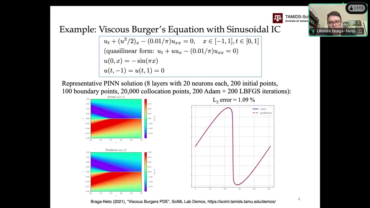
Solving multi-dimensional and more complex partial differential equations (e.g., 2D/3D heat equation, Navier-Stokes, or Burgers' equation) using DeepXDE.
Implementing PINNs to solve inverse problems, such as parameter estimation and system identification from experimental data.
Advanced PINN training techniques, including self-adaptive loss weighting schemes and residual-based adaptive refinement (RAR) to handle stiff gradients.
Exploring Neural Operators (such as DeepONets or Fourier Neural Operators) within DeepXDE to learn mappings between infinite-dimensional function spaces.
5.4K views104likes18:56Original Release: 2024-10-24
hello everyone welcome back to our Channel today we will explore uh one of the most powerful tools for solving differential equations using deep learning that is this deep XDA Library this deep XGA Library so this is the documentation of this Library so this dxg library is a uh python Library designed specially to solve a wide range of differential equations these differential equations can include any type actually so for example if you look at here it can solve ordinary differential equations time independent partial differential equations time dependent equations integral differential equations fractional partial differential equations overall you can solve many types of uh differential equations using this uh D XDA Library so what makes it unique is its ability to handle complex boundary conditions and initial conditions and another thing is the support of these many uh neural network libraries as backend for example with DPX Z you can use tensor flow P torch Jacks paddle paddle so you can use uh any of this uh as your neural network back end today in this tutorial we will walk through the basics of this Library understand its basic syntax and then solve one example this example poison equation in 1D step by step to see how we can use it in practice before we jump into this uh actual coding we need to first set up this uh environment because if you want to run this jupy or notebook in your system you have to set up this environment appropriately so that you can run this juper notebook in your machines as well let's look at that so the process is simple here in this tutorial I'm running this uh juper notebook from my WSL environment I have installed uh this D XTA library and supporting pytorch and other tensorflow libraries within this WSL and from there I'm calling this juper notebook and using them but this works exceptionally well on Windows machines Linux machines other Linux machines MacBooks everything but when you wish to use Linux sorry when you wish to use Windows machine we have a limitation with tensor flow because tensor flow normal tensor flow will work but if you want to use a gpus with tensor flow that will not normally work in the Windows machine either you have to use Linux machine or if you want to use a Windows machine you have to compulsorily install WSL there's no other alternative but for pych and Jacks paddle paddle there's no problem you can use in any machines actually but py and this tensor flow are twoo popularly used libraries so I don't know how far Jack and paddle paddle supports this uh DxD library but you can expect a good support for this py toch and a tensor flow so before installing this uh DP XD you have to install this tensor flow and this py torch so the process is simple open your anaconda prompt just type P install torch or pip install tensor flow anyone either torch or tensor flow is sufficient you don't need to use both after installing this uh tensor flow or py touch you have to use this uh DxD Library which you can install using this pip install dxt command just uh write this in the Anaconda prompt if you are using WSL you can just directly type here or if you are using Windows then you have to install your library via pck package uh from this anakonda prompt there are many ways you can directly install it from jupy notebook as well that's not a problem but this is the way to install this uh DPX but after installing this uh DPX and uh tensorflow and pytorch you have to install some other dependencies like mat plot lib numai Library psyit learn uh pyit optimize scipi so these functions you can install the latest versions no problem you can just uh uh go ahead with Pip install M plot Li pip install numai pip install psyit Lear like that okay and post that here if you want to use this DPX from your Docker image so you can follow these instructions after that you have to set this uh backend variable so as I said this DxD Library works with both py TCH and trans FL right so what you wish to use if you wish to use p torch as your back end then you have to set that variable if you used to use tensorflow as your back end then you you need to set that variable how to set that so here uh they have given some instructions so here you have to set this uh DD backend variable with this uh variable tensorflow do compare. V1 if you want to use tensorflow 1X if you want to use tensorflow 2x you have to set this DD backend variable this is your environment variable keep that in mind so we have to set that with tensor flow and and follow some additional instructions here and uh if you want to use py torch you have to set up this one so you don't need to worry about uh these kind of backend supports because in the coming tutorials whenever we are using pytorch we will uh discuss this in detail before the start of the tutorial no need to worry now let's dive into our example so this is the differential equation that uh we are solving in this tutorial d ² y by DX s + PK s sin PX equal 0 this we are going to solve in this domain minus1 comma 1 and these are the boundary conditions so if you look at this domain so this is our minus one end and this is our one end so here it is our zero origin so at this end our Y is equals to Z similarly at this end our Y is again zero and internally our y solution varies and how it varies so this is our exact solution YF x equal to sin pix these two matte plot lib and nump are two general libraries for plotting and some array and Matrix manipulations and these two libraries are very important first after installing this uh uh dxt Library we have to import it here like this I'm installing this as a DD alas so here I'm setting the back end of this uh deep XDA variable like this from D XDA do backend input TF but this will not work with uh for other tools like py torch Jacks and other things so this is a simple way to set back end if you're working with tensor flow and for other thing py torch and all so we will discuss about them in the coming tutorials whenever we are using py torch we will discuss that in detail and next um the first and a fundamental step in any physics inform neural network is to appropriately Define our main governing differential equation that we are defining it like this using this uh PD function so here I have C clearly defined uh the explanation about what this function does is this PD function uh defines this uh differential equation and it takes two arguments basically X and Y and it returns this residual value that's it and how we are going to do that is with this uh uh grad do hen function so hian function calculates the second derivative of y with respect to X those two we are given here actually so this is our main output quantity and this is our input quantity so in this hn function we are going to evaluate the second derivative of y with respect to X and after evaluating this Dy by DX squ so the remaining quantities like uh pi and sin pix doesn't require any derivatives all we have is the only one second order derivative here that we are evaluating in this hn function and after that after div after setting up this governing differential equation next we need to Define this geometry and the geometry we are defining using this uh geometry module of this uh D XDA Library within the geometry module we have a function called interval so this interval starts from minus1 and end set minus one so that is how we set this geometry that's it and remaining the coordinate generation everything this uh DxD Library will take care on your behalf earlier while generating the collocation points we have defined everything in detail for example here we defined this uh collocation points using this minus1 comma one 100 points we have generated using this Lin space but this is how we Define the geometry earlier but now with the DxD you will just have to define a syntax like this so it will Define your one-dimensional geometry within minus onea 1 boundary and that is stored in this geometry object after setting up this geometry object we need to define the boundaries so boundary means it has two parts actually so what are those two parts so when you take up a boundary it has two things one is the input value and the other one is the output value so given a series of points between minus1 and 1 you have to check whether the given point the x coordinate is existing on the boundary or not if it is existing on the boundary then we need to set its y Val value to zero means the output quantity the solution to zero if it is not on the boundaries then we don't bother about uh the uh output quantity similarly here we need to Define that how we are going to Define it is this way so first we are setting up this boundary so boundary means it takes the x coordinate and a special Boolean variable called on Boundary as I defined here x is the spatial coordinate on Boundary is a Boolean variable means it returns true or false if the x is on the boundary then it returns true else it returns false that's it so that is what this boundary function does and the value of output for example if the input value is on the boundary what is its value so in our case it is zero so that's what we are doing here in this boundary function so here we are setting if the value is on the boundary then we set this to zero and uh this is the exact solution so it it is a sin pix this is our exact solution after defining this so here we are setting up this boundary condition so in DxD there are many ways to set up different varieties of boundary conditions like you have diget B's you have nyman BS you have Robin BS you have hard boundary conditions soft boundary conditions periodic boundary conditions there are many sets of boundary conditions actually for each type of boundary condition D XDA supports certain class of uh functions under this uh ICBC module okay so when we are setting up digate boundary condition those are essential boundary condition we have to use this diget BC from this ICBC module okay this diget BC takes these arguments as primary arguments so what it takes is the geometry and the boundary function and the boundary values so what it does is it will check whether what coordinates within this geometry are on the boundary and and whatever the coordinates that are on the boundary it will use this boundary function to set their final values and next is the this one PD just like we set up this uh boundary conditions we need to Now set up the actual uh governing differential equation that we will do using this PD function this PD function takes these as the primary arguments okay it takes the geometry and the PD itself and here the PD is a function and the BC and this BC is this okay and here these 16 and two points are the collocation point numbers 16 are the number of uh training points that we are going to use in this uh physics informed neural network me these are number of basically the collocation points within the domain and these two are the boundary points boundary points are just two right one is on the left side of this domain and the other one is on the right side of this domain that's it only two points and next this exact solution has no use in the training process why we need this exact solution is because to evaluate the error uh after the training is done and mainly to evaluate this uh metric and this L2 relative error is evaluated with respect to the original exact solution if you don't have for example some differential equations if you want to if you trying to solve you don't have any exact solution you can skip this so if you skip this then you have to skip this uh L to matric also so this this is the link and after that uh these are the number of uh test points so once you define this boundary condition and uh data objects then we have to Define our basic things actually so this is our neural network size and this is the activation function that we are setting up and this is the initializer and this is the net fnn means fully connected neural network okay let's see what are these here this layer size definition is very important and tricky also here if you look at here so our network has one input layer and one output layer and three hidden layers each layer with 15 neurons so that is what we are defining here so this is a kind of uh encrypted expression so if you define like this you will get the output like this actually so keep this in mind for example if you want to extend this uh Network to say to use uh 20 neurons in each hidden layer instead of 50 and increase the number of layers from 3 to 10 maybe you just have to replace these numbers so this with u 20 and this with 10 that's it it will create a new list with uh 1 20 20 20 20 with the 10 values of 20s and then one that's it so this is how the list will be generated so this is a little uh interesting thing and but this is how dxt library is using its syntax to define the layer size and uh just like activation function DxD supports all sorts of activation function you can use anything tan sigmoid reu P you can use everything and this is the GL rot uniform initializer so what it does is it initializes the weights and biases during the start of the uh training and next uh with these quantities we will initialize this uh FN and fully connected uh neural network from this NN module of this dxt after setting up uh these things we will now initiate our model objective model we are initializing with this model module from for this we are sending the inputs as a data and net after this model object is initialized then we are setting up this uh compile function so here for the compile we are sending this uh Adam Optimizer and the learning rate as 0.1 and Matrix we are setting as L2 relative error this uh dxt supports other types of Errors other types of optimizers as well but since it is a introductory tutorial my objective here in this tutorial is to give you a overview rather than going into specifics of each object which we will do in the coming tutorials so after this model definition is done we are going to train the model for thousand EPO here iterations refers to the number of epo okay model. Trin does the training purpose so once you to do this and run your analysis so you will see a training information like this actually so this training information gives you main three important things one is the train loss test loss and the test metric So based on these numbers you will verify whether your overall training is good or not so after the at the end of thousandth Epoch or iteration these are our values train loss is of the order of 10^ minus 5 test loss is of the order of 10^ minus 4 and the test matric is of the order of 10^ minus 4 these are fantastic and good so in this tutorial we have an analytical solution so you can definitely use it for benchmarking your PIN solution but in the cases where analytical solution or reference solution is not available then you have to solely rely on the main governing differential equation and the boundary condition satisfaction actually so there evaluating just this final value is not suff ient because you don't have this uh reference points right so in that case you have to look at few more quantities like your boundary condition satisfaction residual satisfaction so after training your model this is where we are uh visualizing our results actually so if you use this uh uniform points from this uh J module so what it gives you is it will give you a set of X points within the domain minus 1A 1 so here we setting up the number of points 30 so if you use uh 20 points so it will give you a plot like this okay meaning it just consider 10 20 points if you give Five Points like this so the shape of the curve is also different so we have to use some decent number of points to exactly represents the sign function okay and after that these are our general mat plot lib commands so this is how we use uh deep XD for solving this uh basic example of uh poison equation in 1D with this dxt Library there are some additional advantages like uh for example you can generate this kind of uh animations as well so here the black line uh represents the original solution and this uh Red Line represents your training solution you can get this kind of uh beautiful animations which you can present them in your uh desertation seminars so this solution that corresponds to this Oiler beam so which we will solve in our next tutorial using D XTA this tutorial we are going to learn some other Concepts like applying nman BC and some other General boundary conditions apart from the dlet and N B's okay and also we are going to look at another form of uh derivative first order derivative evaluation using this uh Jacobian okay that's it for this tutorial uh see you in the next tutorial thank you happy learning
Up Next

20:53
How to Create Your Own Academic Corpus with AntConc
@DrRonMartinez
146 views•2020-06-12

178:38
Whole Brain Architecture: First International Workshop 2024
@thewholebrainarchitecturei9784
640 views•2024-07-22

9:49
FastAPI vs Flask vs Django: Choosing the Right Python Web Framework
@TechWithTim
302.5K views•2024-05-26

1:42
Game of Thrones Opening Credits: A Cinematic Analysis
@gameofthrones
46.3M views•2011-04-18
Related Study Plans & Knowledge Roadmaps
Structured learning paths in General & Interdisciplinary Studies
general-studies
Artificial Light: History, Tech & Human Impact
01The Pre-Electric Era: Fire, Oil, and Gas Lighting
02The Incandescent Revolution and Grid Electrification
03Gas Discharge and Fluorescent Illumination
+ 3 more learning modules
14h6 modules
Explore Roadmap
general-studies
Elevator Engineering: History, Physics & Cities
01From Hoists to Safety Brakes: The Dawn of Vertical Lift
02Hydraulic vs. Traction: The Engineering Physics of Elevators
03Modern Speed, Safety, and Algorithms
+ 2 more learning modules
12h5 modules
Explore Roadmap
general-studies
Rubber: Material Science, History & Geopolitics
01Origins of Natural Rubber & Mesoamerican History
02The Chemistry of Natural Rubber & Vulcanization
03The Geopolitics of the Rubber Boom & Colonization
+ 2 more learning modules
12h5 modules
Explore Roadmap
general-studies
Containerization: Evolution, Logistics & Trade
01Ancient Trade & Bulk Cargo: Amphorae to Barrels
02The Industrial Revolution & Cardboard Packaging
03The Containerization Revolution: Malcom McLean
+ 2 more learning modules
12h5 modules
Explore Roadmap