![[線性代數] 第1-1 單元: Introduction to Linear Algebra](https://i.ytimg.com/vi/IG-EQUIk7P0/maxresdefault.jpg)










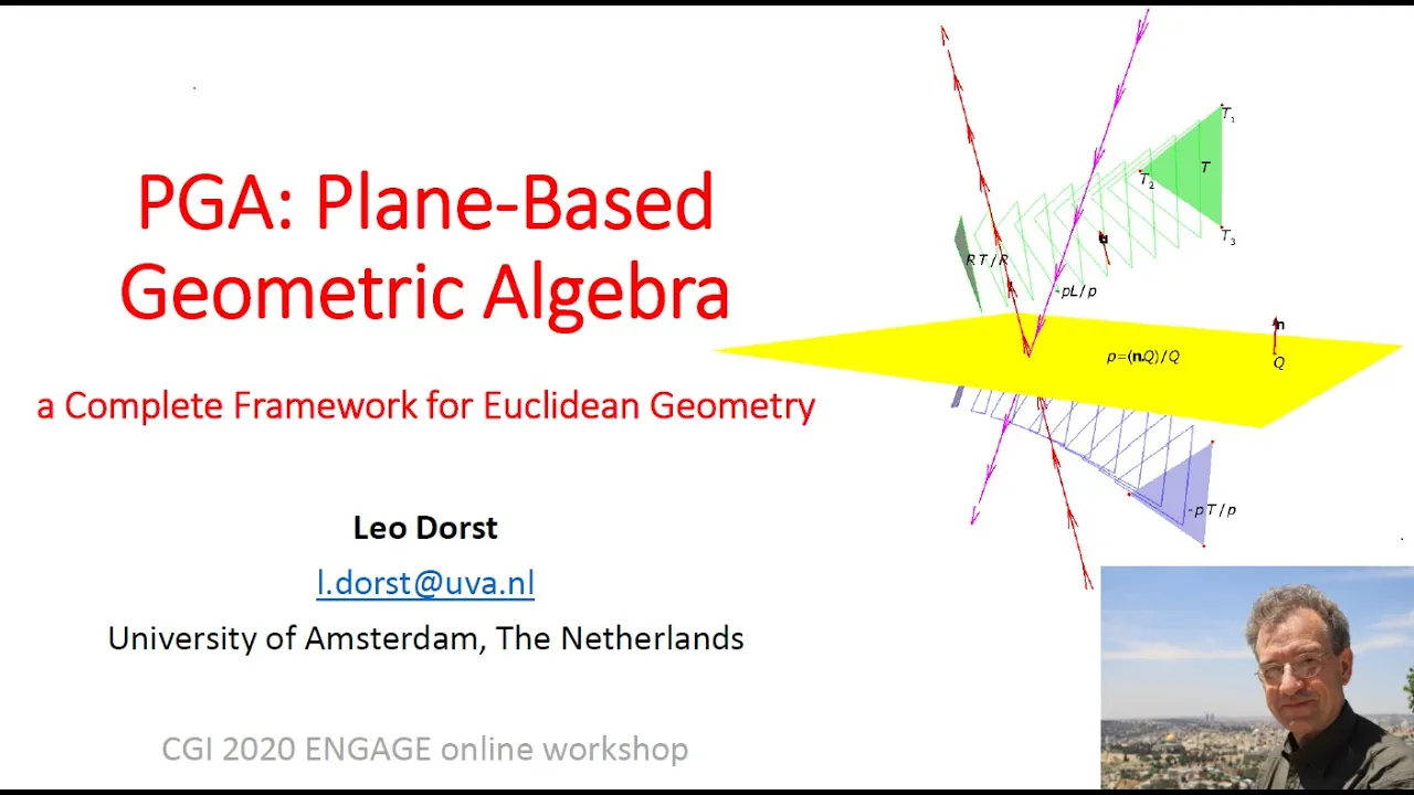




Projective Geometric Algebra (PGA) is a powerful mathematical framework that unifies fundamental geometric operations—meet (intersection), join (connection), projection, and rigid transformations—into a single, dimension-independent system. In PGA, geometric objects like points, lines, and planes are represented as multivectors within a geometric algebra structure, where the outer product computes intersections, the regressive product computes joins, the inner product enables projections, and the sandwich product applies transformations. This approach simplifies complex geometric computations by replacing dozens of separate formulas in traditional vector algebra with a few unified operations that work consistently across any dimension, making it particularly valuable for computer graphics, animation, and computational geometry applications.
Projective Geometric Algebra Explained: A Swift Introduction
Added:Have you ever wanted to calculate reflections, rotations, and translations?
What about joining two objects together or finding the intersection of two objects, including being able to handle some of the annoying edge cases?
What about projections?
What about being able to do all of this in any number of dimensions?
Could there really be a mathematical system that can easily do all of these things?
There is!
This video is an introduction to projective geometric algebra, or PGA, which is a flavor of geometric algebra that can easily do all of these things and more.
In PGA, we turn this into this, this into this, and all of this into this.
Before we get started, I need to clarify the term "projective geometric algebra".
The reason for this name is that it was initially described as combining geometric algebra with projective geometry.
However, later on, people started realizing other ways of developing PGA that skip the projective geometry, such as using geometric algebra to describe rigid transformations, or by directly doing geometric algebra on the linear space of lines or planes.
In this video, we will be taking this third route, where we directly do geometric algebra on the linear space of lines or planes.
Thus, despite this video being called "A Swift Introduction to Projective Geometric Algebra", we won't actually be doing any projective geometry.
If you want to see one of these other approaches to PGA, I'll leave some links in the description that you can check out.
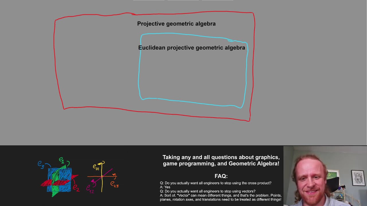
Another thing that I need to point out is that PGA is not limited to Euclidean geometry.
We can do elliptic PGA and hyperbolic PGA as well.
However, in this video I will only focus on Euclidean PGA, mainly for the sake of time and because it is the one that I am the most familiar with.
Also, at certain points in the video, I'll be skipping some details for the sake of speed and clarity.
At some of those moments, you will find a note on the bottom right of the screen.
A corresponding note will be in the description explaining the skipped details.
Well, without any further ado, let's get started.
Our foundation will be the linear space of lines.
I made a video covering this linear space, uh, some time ago, but in case you haven't seen it, I'll briefly go over the important features of this linear space here.
To make lines into a linear space, we write the equations for the lines in this form.
To make it easier to use lines as vectors, we use a basis that we call e one, e two, and e zero, and then we associate lines with linear combinations of these three vectors.
Using this notation, the horizontal line here is e two plus e zero, while the slanted line is e one minus e two plus e zero.
e one is the vertical line through the origin, e two is the horizontal line through the origin, and e zero is the line at infinity.
With this basis, we can add and scale lines just like any other kind of vector, by adding and scaling the components.
We can also find the magnitude of a line with a formula which is like that of the length of an arrow except that the e zero component is ignored.
For example, the magnitude of u is one, and the magnitude of v is the square root of two.
Geometrically, the sum of two lines is a new line that passes through their intersection point.
The slope of this line is found by the relative magnitudes of the two lines being added.
The higher the magnitude of one line, the closer the sum gets to that line.
With the right coefficients, we can reach any of the lines that go through the sum.
Also, adding scalar multiples of e zero corresponds to shifting the line.
One other interesting thing about this linear space is that scaling a vector doesn't change what line it represents.
For example, this line here is represented by the vector e two plus e zero, but the vector two e two plus two e zero also represents this same line.
This feature is going to be true for all PGA objects, so keep it in mind.
In general, the geometric objects the algebraic objects in PGA represent won't change if you scale them by a nonzero value.
If you want to see more details about this linear space, I would suggest watching my video on the subject.
One aspect of this linear space that I did not mention in that video is the inner product.
From the formula for the magnitude of a vector, we can derive a formula for the inner product of two vectors.
It looks like the usual inner product, except that because the e zero component doesn't contribute to the magnitude, it doesn't contribute to the inner product either.
Geometrically, the inner product of two lines is equivalent to the inner product of two arrows.
For example, like with arrows, the inner product of two lines is equal to the magnitude of the two lines times the cosine of the angle between them.
Furthermore, because the e zero component doesn't contribute to the inner product at all, we can shift these lines around without changing this result!
Using the inner product, we can define what it means for two lines to be parallel or perpendicular as well.
Two lines are perpendicular when the cosine of theta is zero, which means that their inner product is zero.
Two lines are parallel when the cosine of theta is one, which means that their inner product is the product of their magnitudes.
Actually, two lines are also parallel if the cosine of theta is negative one, which we can account for by throwing in an absolute value.
While it may seem like these ideas are the same as for arrows, there are a few notable differences.
First, because the inner product of any vector with e zero is zero, we can see that e zero is both perpendicular and parallel to all vectors, similar to the zero vector.
The second difference relates to this condition for being parallel.
Traditionally, this equation only holds when one vector is a scalar multiple of the other.
In the linear space of lines, multiplying by a scalar doesn't change a line, so it would seem that only vectors that represent the same line are parallel.
However, that's actually not the case.
If we have the inner product of a line with a scalar multiple of e zero plus itself, after distributing, the second term disappears because it's an inner product with e zero.
Now because all vectors are parallel with themself, this is the product of the magnitudes.
And because the magnitude of e zero is zero, we are able to add the scalar multiple of e zero back in.
Thus, these two vectors are parallel, despite not being scalar multiples of each other.
Geometrically, because adding scalar multiples of e zero shifts the line, what we have shown here is that in the linear space of lines, the geometric and algebraic definitions of parallel and perpendicular agree.
Now that we've reviewed the linear space of lines, we can finally see what PGA actually is.
PGA is the geometric algebra built from the linear space of lines.
Well, this is actually just two-dimensional PGA.
We'll see how higher-dimensional PGA works later.
Now I realize that some of you may have come upon this video without really knowing anything about geometric algebra.
I have made many videos about geometric algebra in the past, and you can find some of them in the description.
However, if you're willing to fly by the seat of your pants, you could probably get away without watching those videos.
While you may not understand exactly how the operations we will use are exactly defined, you should still be able to understand the general idea of what's going on.
In two-dimensional PGA, we have scalars, vectors with three components e one, e two, and e zero, which represent lines, bivectors with three components e zero e one, e zero e two, and e one e two, which represent two-dimensional subspaces of lines, and trivectors with one component, e zero e one e two.
As I've said before on this channel, to make the notation a little neater, we often write bivectors and trivectors as a single e with several subscripts, which we take to mean the product of those several basis vectors.
Together, these multivectors are what make up PGA.
Now one interesting thing to note is that while we are working in two-dimensional space, algebraically, this is a three-dimensional geometric algebra.
Thus, many of the features of three-dimensional geometric algebra will be present here, even though we are working in two-dimensional space.
Now to calculate the geometric product, things are mostly the same but with one important difference.
Like usual, the product of different basis vectors anticommutes.
However, things are a little different when it comes to what the basis vectors square to.
In geometric algebra, the square of a vector is its magnitude squared.
We already know that the magnitude of a line is given by this equation.
Thus, while e one and e two square to one, it turns out that e zero squares to zero.
And that's it!
Everything we will do in this video can be derived from what is on the screen right here.
We will also be using other products like the outer product, the regressive product, and the inner product, but those can be defined in terms of the geometric product.
Really, all of the power in PGA follows from just this.
Now that we understand what PGA is at its core, let's start exploring its content.
Let's start with understanding bivectors.
In geometric algebra, bivectors represent two-dimensional subspaces.
But what exactly is a two-dimensional subspace in the linear space of lines?
Well we can think of a two-dimensional subspace as being the span of two vectors.
In geometric algebra, the span of two vectors is represented by their outer product.
So to understand bivectors, let's look at the span of two vectors, which will also give us an idea of what the outer product does.
Here's two vectors.
What is their span?
Well in the linear space of lines, every linear combination of these two vectors will pass through their intersection.
And with the right choice of coefficients, we can reach any of the lines that pass through this point.
This shows us that the span of these two vectors is every line that passes through this point.
Thus, we can think of bivectors as representing the set of all of these lines.
But honestly, if you ask me, thinking of this whole set at once is a bit difficult.
Is there something simpler that we can use?
Well the set of all lines passing through a point is uniquely determined by that point.
So what if, instead of thinking of this bivector as being all of these lines, we instead think of this bivector as just being the one single point that all the lines pass through?
This point is much easier to conceptualize than that monstrous set of lines.
Furthermore, this gives a surprisingly simple geometric picture of the outer product in PGA: the outer product of two vectors is simply their intersection.
Wait, hold on.
We can't just start saying that the outer product is the intersection!
The intersection of two lines and the outer product are both operations that have already been defined completely independently of each other, so they can't possibly be the same thing, right?
Well, let's check.
Let's say we have two arbitrary lines a and b.
Remembering that these vectors correspond to linear equations, you can solve this system of linear equations to get the coordinates of the intersection point.
Now to calculate the outer product, we will expand the definitions of a and b and use these equations for the outer product to simplify.
Like with any product, we start with distributing.
Honestly, this expression is ridiculous, so let's try to simplify it.
First, because the outer product of a vector with itself is zero, we can remove these three terms.
We can now swap a few of the products at the cost of a minus sign.
Now the outer product of two different basis vectors is just their geometric product, which makes things look a little neater.
Rearranging a bit, we can see that we can factor out the basis bivectors.
Thus, we see that the outer product is not the interse - no, wait a minute... These expressions look suspiciously similar!
Looking at them, we can see several parts that are the same.
In fact, because scaling multivectors in PGA doesn't affect what geometric object they represent, we can divide the result by the e one two coefficient to make the other coefficients precisely the coordinates of the intersection point!
What this shows us is that points in 2D space do in fact correspond to bivectors in 2D PGA.
This might all seem really complicated, but that's because the normal way of finding intersections is complicated.
If we forget about the normal way of finding intersections, the result is very simple.
Under this correspondence between bivectors and points, we have seen that the intersection of two lines is simply their outer product.
In geometry, this operation is often called the meet, because it finds where two lines meet.
Thus, in 2D PGA, the meet is represented by the outer product.
Also, we know that in geometric algebra, the geometric product of two perpendicular vectors is the same as their outer product, meaning that when two lines are perpendicular, their meet is also their geometric product.
Now I want to look at this correspondence between points and bivectors in more detail.
Given an arbitrary bivector in 2D PGA, we can find what point it represents by simply dividing by the e one two component, which in PGA is actually just normalizing the bivector.
Let's look at some examples.
This bivector simply corresponds to the point two, one.
If the e one two component was one half instead of one, the point it corresponds to would be four, two, because we would have to divide the bivector by one half to normalize it.
Now one question you might be asking is what about bivectors with no e one two component?
We can't normalize this bivector, so what point does it represent?
Let's try to figure this out by letting the coefficient of e one two approach zero.
As the coefficient of e one two gets closer to zero, the point shoots off to infinity.
This looks similar to the situation when we are approaching the line at infinity, so we say that bivectors that have no e one two component are points at infinity.
Interestingly, unlike with the line at infinity, we have many different points at infinity, one for every possible direction.
Like the line at infinity, points at infinity can be very useful at times.
For example, what is the meet of a line with the line at infinity?
Geometrically, I would think that it's the point at infinity in the direction of the line.
The direction that an arbitrary line goes in is b, negative a.
Let's check to see if calculating the meet here will produce the point at infinity in this direction.
Thus, we see that the meet of a line with the line at infinity is in fact the point at infinity in the direction of the line.
Another situation that we can work out now is the meet of two parallel lines.
Calling one of these lines a, we can write the other line as a plus some scalar multiple of e zero.
Then when we calculate their meet, the first term disappears because the outer product of a vector with itself is zero.
This leaves just the meet of the line with the line at infinity, and we just showed that this is the point at infinity in the direction of the line.
Thus, the meet of two parallel lines is the point at infinity in the direction that the lines are going.
If we change our perspective slightly, we can see that this result makes sense geometrically as well, because parallel lines converge to the same point on the horizon.
The next thing I want to talk about is the regressive product.
In 2D PGA, the only interesting case to look at is the regressive product between two points.
The regressive product between two objects is their common subspace.
What is the common subspace of these two points?
To figure this out, we need to remember that a point actually represents all of the lines going through that point.
So what's the common subspace of these two subspaces?
Well, we have to find what lines are in both subspaces.
To be in the subspace of a point, a line has to pass through that point, so to be in both subspaces, a line has to pass through both points.
There's only one line that passes through both points.
Thus, we see that the regressive product of two points is the line joining the two points.
Now I want to compare this way of finding this line with the traditional way.
Given two points with these coordinates, the equation for the line going through them can be found using the point-slope form of a line.
If we wanted to, we could do a bit of algebra to convert the equation to the general form.
So this is the equation for the line that joins the two points.
But in PGA, we don't have to mess with the components at all, and we can just write this line as the regressive product of the two points.
In geometry, this operation is often called the join, because it finds the line that joins the two points together.
Thus, in 2D PGA, the join is represented by the regressive product.
Now that we've explored the meet and the join, the next thing I want to look at is the inner product.
While we've looked at the inner product of vectors already, in geometric algebra, the inner product is not limited to just vectors.
What about the inner product of two bivectors?
Well, if you work out the inner product of these two bivectors, it actually ends up just being negative a three times b three.
Because we often want a three and b three to be one, this means that the inner product of two bivectors is honestly not that interesting, so we won't look into it any further.
However, what about the inner product of a vector and a bivector?
This is where things really get interesting.
To calculate the inner product of a vector and a bivector, we project the vector onto the bivector and then contract.
To do this in the context of PGA, we need to think of the point as being all of the lines going through the point again.
We first project the vector onto the bivector, and then the contraction removes all of the lines that have any horizontal component.
Thus, we see that the inner product of a point and a line is the perpendicular line passing through that point.
Note what happens if the point is actually on the line.
We know that the geometric product of a vector and a bivector is the sum of their inner and outer products.
Because the point B is on the line a, we can write B as the meet of a and the vertical line.
We now have the outer product of a vector with itself, so this term disappears.
All that's left on the right-hand side now is the inner product.
Thus, we see that if a point is on a line, their geometric product is equal to their inner product.
The inner product is useful for finding some other things as well.
For example, because the inner product is perpendicular to the original line, we can multiply them to get their intersection point, which is the projection of the original point onto the line.
Also, if we multiply the inner product with the original point, we get the line parallel to the original line going through the point, because as we just saw, the product of a line and a point on the line is their inner product.
Looking at these two formulas, they are remarkably similar.
Geometrically they are doing similar things too.
In one case, we are projecting the point B onto the line a, while in the other case, we are projecting the line a onto the point B.
So in the end, we can do either projection with just this simple formula, no matter which object we're talking about!
If you think this looks familiar, that's because this is practically the same thing as the usual projection formula for arrows!
The only difference is the inverse in the second formula.
However, since scalar factors don't change what object a multivector represents in PGA, we are free to drop the inverse in PGA, and it is usually simpler to do so.
Like with the meet and the join, I want to compare this with the traditional ways of calculating projections.
Given a point and a line, the projection of the line onto the point will have the same slope, so the x and y coefficients will be the same, but we want the line to pass through the point x zero, y zero.
After a bit of simplification, we get this.
While projecting a line onto a point is simple, projecting a point onto a line is not.
I looked it up, and people only described a process for doing it that I learned years ago, and not an explicit formula.
Thus, I worked out the formula myself, and I can see now why people never use it.
Looking at these two formulas, they seem to be describing completely different, but in PGA both kinds of projections are described by the same simple formula!
If you don't believe me, try it out for yourself!
Calculate this expression for arbitrary vectors and bivectors and you'll find that you get the exact formulas shown here for projecting a line onto a point and for projecting a point onto a line.
Now that we've talked about the meet, join, and projections, I want to move on to discussing the most important part of PGA: the geometric product.
I showed earlier how we calculate the geometric product in PGA, so I want to focus now on what we can do with it.
If you've seen my videos before, you'll know that I like to focus on three things when it comes to the geometric product: two-dimensional rotations, reflections, and orthogonal transformations.
You may think that we'll start with the two-dimensional rotation formula because we're working in two-dimensional space, but there's a problem.
I said previously that even though we're working in two-dimensional space, two-dimensional PGA is actually a three-dimensional algebra.
This means that except in certain subspaces, the two-dimensional rotation formula does not hold.
So instead, I'll start with focusing on the reflection formula.
Let a and u be vectors.
To calculate this product, we can decompose u into two pieces, one which is parallel to a, and the other which is perpendicular to a.
By distributing, we can consider the product of the parallel and perpendicular parts separately.
For the parallel part, u parallel and a represent the same line, so their product is a scalar.
Thus, u parallel a u is a scalar multiple of u, so it represents the same line.
For the perpendicular part, because u perpendicular and a are perpendicular, their product is their meet.
Because the product of a line and a point on that line is their inner product, u perpendicular a u is this vertical line.
Now we need to add these two lines.
To do so, notice that because u parallel and u perpendicular were both multiplied by the same thing, the relative magnitude of u parallel a u and u perpendicular a u is the same as the relative magnitude of u parallel and u perpendicular.
u is closer to u parallel than to u perpendicular here, and the sum will be that close to u parallel a u as well.
In particular, the angle between u and u parallel is the same as the angle between the sum and u parallel a u.
I'll admit that this argument is a bit hard to follow, but the important point is this: we have reflected a across u, so the sandwich product still represents reflections in PGA.
Armed with this reflection formula, we can start describing many other kinds of transformations.
For example, like usual in geometric algebra, two reflections is the same as a rotation around the intersection point of the two vectors by twice the angle between the two vectors.
Like usual in geometric algebra, we call the product of an even number of vectors, such as u v here, a rotor.
Well actually the usual definition of rotor requires the vectors to be normalized, but in PGA we don't usually need to bother with normalization so I'll be a bit lax on the terminology here.
We can write the rotor as its own variable R, which allows us to write the rotation formula like this, where the dagger represents the reverse of a multivector, which corresponds to reversing the order of vectors in a product.
Now, if two reflections is a rotation around the intersection point, you might be wondering, "What about two reflections across two parallel lines where there is no intersection point?"
Well, recall that two parallel lines meet at a point at infinity.
What would a rotation around a point at infinity look like?
Let's find out.
To do so, we can pick an arbitrary line a and see how the two reflections affect it.
We see that instead of rotating, reflecting across two parallel lines has translated the line.
In fact, it's not too difficult to prove that the distance the line moved is twice the distance between u and v.
So we see that a rotation around a point at infinity is simply a translation!
If you think about it, this should make sense.
The further away you are from the center of rotation, the more a rotation looks like a translation.
Thus, when the center of rotation is infinitely far away, the result is a translation.
In PGA, people sometimes use the term motor instead of rotor to emphasize the fact that we can represent translations in addition to rotations and only use the term rotor for the motors that represent rotations, although I personally don't do so.
With enough reflections, we can represent, compose, and apply any rigid transformation on the plane.
Wait, hold on.
When we think of transformations in space, what are we usually transforming?
That's right, points!
We've been playing with lines this whole time, so how can we say that we can represent any rigid transformation if we can only manipulate lines, and not points?
Well, points are a thing in PGA, so let's look into how to calculate these transformations on points in PGA.
Since all rigid transformations can be written as the composition of reflections, let's figure out how to reflect a point across a line a.
To figure this out, notice that we can write the point as the geometric product of two perpendicular lines u and v.
Now, if we reflect u and v, we can see that the reflection of the point across a is simply the meet of a u a and a v a.
In fact, a u a and a v a are still perpendicular, so this is actually just their geometric product.
We now have a scalar factor of a squared, which we can drop because scalar factors don't affect what point the bivector represents.
Now that we've figured this out, I'll forget about the lines we used to get here and just call the point P.
So this is the formula for reflecting a point in PGA.
Wait a minute... This is exactly the same as the formula for reflecting lines!
What we see here is that the reflection formula works no matter what multivector we are working with!
And because we can build all rigid transformations out of reflections, we can now describe all rigid transformations on both lines and points using the same simple formula.
The last thing that I want to look at in two dimensions is the exponential form of rotors.
In geometric algebra, we often like to represent rotors as exponentials of bivectors, so what does that look like in PGA?
Well in 2D PGA, bivectors are points.
What does the exponential of a point look like?
To figure this out, let's think of this point as being the product of two perpendicular lines u and v.
Now, unlike usual in PGA, the magnitude of the argument of the exponential actually matters, so to make things simple, let's assume that u and v are unit vectors.
Because they're perpendicular unit vectors, the product u v squares to negative one, meaning that we can expand the exponential using Euler's formula.
Now because u is a unit vector, we can multiply the first term by u squared, which allows us to factor out u.
From this, we see that this exponential is a product of two vectors, so it is a rotor.
In fact, because u and v have the same magnitude, they add similarly to vectors, which means that the second vector in this product is just u rotated by the angle theta.
All together, this means that when we use this exponential in a sandwich product, the result is just a rotation by two times theta around u v!
Thus, exponentiating a point produces a rotation around that point.
We can use this to rotate around an arbitrary point P at an arbitrary angle theta.
Now, you might be wondering, what about exponentials with points at infinity?
We can figure this out as well.
As we saw before, we can think of a point at infinity as being the meet of a vector with the line at infinity.
Because the line at infinity is perpendicular to every vector, this is equal to the geometric product of the two vectors.
So what happens if we raise e to this point times some parameter x?
Well unlike before, because it has a factor of e zero in it, the argument squares to zero rather than a negative number, so Euler's formula no longer applies.
So what can we do here?
Well, if we expand the exponential using its Taylor series, we see that every term after the first two has a factor of u e zero x squared, so all of those terms are zero.
At this point, we can proceed with the analysis similar to before.
Because u is a unit vector, we can multiply the first term by u squared, which allows us to factor out u.
Once again, we see that this exponential is a product of two vectors, so it is a rotor.
In fact, because u is a unit vector, adding x times e zero simply shifts the line by x.
All together, this means that when we use this exponential in a sandwich product, the result is just a translation by two times x perpendicular to u!
We can use this to translate around an arbitrary point at infinity P by an arbitrary distance x.
Once again, we see that in PGA, rotations and translations are practically the same thing.
Like with every other operation we've looked at so far, I want to compare this with the usual way of calculating rigid transformations.
Traditionally, we think of reflections and rotations as being orthogonal transformations.
We represent these orthogonal transformations using things like rotation matrices, complex numbers, or quaternions.
As for translations, we usually use vector addition.
There are two main issues with the traditional ways of doing these operations.
First, because rotations and translations are calculated using completely different operations, composing them can be annoying.
But in PGA, because both rotations and translations are rotors, we can compose them simply by multiplying them.
In fact, we could just define a new rotor R that is equal to R one R two R three, making applying several rotors exactly the same as applying a single rotor.
The second issue with the traditional way of doing things is an even bigger problem than the first.
Consider a vector.
We can rotate it all we want using one of the previously mentioned methods.
However, we have one important limitation: we can only rotate around the origin!
If we wanted to rotate around another point represented by a vector p, the conventional way to do this is to subtract p from v, do a rotation around the origin, and then add p again.
But in PGA, rotations don't care about what point they're rotating around.
Every rotation, no matter what it's around, is given by the same simple formula.
Let's summarize what we've learned.
Calculating the meet, or intersection, is just the outer product.
Calculating the join is just the regressive product.
Calculating projections, no matter what objects we're talking about, is this formula involving the inner product.
And finally, calculating rigid transformations on any kind of object is just the sandwich product.
And that's it!
These few simple operations open up the way to a myriad of geometric applications.
However, up until this point, we have only been focusing on two-dimensional space.
What about three-dimensional space?
Before we start exploring three-dimensional PGA, I want to look at how we traditionally work with three-dimensional geometry.
In two dimensions, our main objects are lines and points.
In three dimensions, while we still have lines and points, we also add a new object: planes.
The addition of a third kind of object brings about many complications.
In two dimensions, we only have one kind of meet to calculate and one kind of join to calculate.
Also, while there are two different kinds of projections, they still both involve the same two kinds of objects.
But in three dimensions, things get much more confusing.
Instead of having one kind of meet, we now have three: the meet of two planes, which is their line of intersection, the meet of a plane and a line, which is their point of intersection, and the meet of three planes, which is their point of intersection.
Similarly, we now have three kinds of joins: the join of two points, which is the line passing through both of them, the join of a point and a line, which is the plane passing through both of them, and the join of three points, which is the plane passing through all three points.
If that wasn't bad enough, we now have *six* different kinds of projections!
We can project a line onto a plane, a plane onto a line, a point onto a plane, a plane onto a point, a point onto a line, and a line onto a point.
The traditional way of performing all of these operations algebraically is to use vector algebra, as long as we can find a representation of planes, lines, and points using 3D vectors.
To represent planes, we can think of them as being a pair of a vector and a scalar, corresponding to the plane given by this equation.
One of the best ways that we know of to represent three-dimensional lines is using something called Plücker coordinates, where we represent a line as a pair of vectors, usually written like this.
Since Plücker coordinates are not the point of this video, I won't go into how these two vectors represent a line.
Finally, we can represent points using just a single vector.
Using these representations, we have three different formulas for the different kinds of meets, three more formulas for the different kinds of joins, and *six* more formulas for the different kinds of projections.
This seems rather crazy, but what can you expect?
Of course the formulas for operations with different kinds of objects would be completely different, right?
There's no reason to think that they shouldn't be.
Anyway, now that we've seen how these problems are solved without PGA, let's look into three-dimensional PGA to see how it handles these problems.
In two-dimensional PGA, our vectors represent lines under this correspondence.
One idea we might have for jumping up a dimension is to just add another basis vector, which would then correspond to an equation like this.
This is the equation for a plane in three dimensions.
Thus, while 2D PGA is based on the linear space of lines, 3D PGA is based on the linear space of planes.
So let's start with briefly looking at the linear space of planes, which is surprisingly similar to the linear space of lines.
In the linear space of planes, we have four basis vectors: three representing the three orthogonal planes through the origin, and a fourth representing the plane at infinity.
A linear combination of two planes is another plane passing through their intersection, and the coefficients say how close to each input plane the result should be.
Like with lines, with the right coefficients, we can reach any of the planes that pass through their intersection.
Like lines, every plane has a magnitude given by this equation, which is again like the usual equation for magnitude but without considering the e zero component.
This equation is what brings us to the definition of the geometric product in 3D PGA: the geometric product of different basis vectors anticommutes, and the basis vectors square to their magnitude squared.
In 3D PGA, we have scalars, vectors with four components, which represent planes, bivectors with six components, which represent two-dimensional subspaces of planes, trivectors with four components, which represent three-dimensional subspaces of planes, and pseudoscalars with one component.
All of this is what makes up 3D PGA.
To start exploring 3D PGA, let's start with figuring out what geometric objects bivectors and trivectors represent.
Like before, we can think of bivectors as two-dimensional subspaces, so let's consider the span of two vectors.
As I said before, the span of these two planes is all of the planes that pass through the intersection of the two planes.
Like in two dimensions, notice that these planes are uniquely determined by the line all of the planes pass through.
Taking a hint from what we saw in two dimensions, let's just say that this bivector simply is the line.
Similarly, for trivectors, we need to understand the span of three planes.
Using arguments similar to those for the span of two planes, you can show that the span of three planes is all of the planes passing through the intersection point of the three planes.
Again, this set of planes is uniquely determined by the point they all pass through, so like in the other cases, let's say that the trivector *is* the point.
Now, if you ask me, seeing all of these planes at once is pretty confusing.
Thus, to make visualization simpler, when I'm talking about all of the planes passing through a point, I'm only going to show three orthogonal planes going through the point.
For similar reasons, I'll also do the same for lines.
When talking about all of the planes passing through a line, I will only show two orthogonal planes passing through the line rather than several planes passing through the line.
Anyway, we see that in 3D PGA, vectors are planes, bivectors are lines, and trivectors are points.
Like in two dimensions, we can also have planes, lines, and points at infinity.
But for the sake of time, I won't be talking about them here.
They behave mostly as you would expect.
Wait, we might have arguments for these correspondences geometrically, but how do these correspondences work numerically?
We know that vectors correspond to planes written in this form, but what about lines and points?
Well for points, we can use similar arguments as in the two-dimensional case to show that this is the correspondence between trivectors and points.
But that still leaves lines.
We know that our bivectors are of this form, but how do we know what line this represents?
For reasons I won't go into here, it turns out that 3D PGA actually uses Plücker coordinates, which I briefly mentioned before, to represent lines.
So does that mean we're going to have to learn Plücker coordinates now?
Surprisingly, no, and in fact, I've actually forgotten how they work at this point!
We can just use PGA to manipulate the lines geometrically, and everything works out.
If you really need to figure out exactly what line a bivector is, it's not too difficult to find two points on the line using PGA operations that I'm about to describe, and you can figure out an equation for the line from that.
Anyway, now that we know what multivectors are in 3D PGA, let's start exploring how to do three-dimensional geometry with it, starting with the meet.
Actually, we have pretty much already figured this one out.
The outer product of two planes represents their span, so the outer product is their meet.
For the same reason, the outer product of three planes is their meet.
The case that's not immediately obvious is the meet of a plane and a line.
However, this is easy to figure out if we realize that we can write L as the outer product of two other planes, showing that the outer product of the plane and the line is the outer product of these three planes.
This point is simply the meet of the original plane and line.
In each case, we've seen that the outer product represented the meet.
Somehow, despite the fact that we have three completely different kinds of meets that traditionally use completely different formulas, in PGA, we use the same operation for all of them!
Also, like in two dimensions, the geometric product of perpendicular objects is equal to their outer product.
Thus, the geometric product of two perpendicular planes is their meet, the geometric product of three perpendicular planes is their meet, and the geometric product of a plane and a perpendicular line is their meet.
Now that we've seen that the meet is easy, let's move on to the join, starting with the join of two points.
We know that the join of these two points is this line.
To try to express this line in terms of the points, let's look at the subspaces these points represent, which are these planes.
Now, notice that of these planes, these planes are the planes that represent the join of the two points.
They are also precisely the planes that are common between the two points.
By definition, the common subspace of two objects is their regressive product, showing that the join of two points is their regressive product.
For a line and a point, this plane is their join.
How can we find this plane in terms of the subspaces that the line and the point represent?
Well, notice that the plane representing the join is again the only one that is common to both subspaces, meaning that once again, the join is the regressive product.
The last case to check is the join of three points.
Fortunately, we can actually figure this out using the previous two cases.
The join of P one and P two is the line joining them, and then the join of this line with P three is this plane.
Thus, we see that the join of three points is, in fact, the regressive product of the three points.
Thus, like with the meet, we use one single operation to represent the join in PGA, no matter what the inputs are!
So far, we have seen that the three different kinds of meets, despite having different formulas in vector algebra, are all represented by the outer product in PGA, which is the same as in two dimensions.
Similarly, the three different kinds of joins have different formulas in vector algebra, but are all represented by the regressive product in PGA, which is again the same as in two dimensions.
Could we possibly hope that the same will be true for projections?
The issue here is that there are now six different kinds of projections.
They can't possibly all be given by one single formula, right?
Well let's check.
But before we can do that, we need to look into the inner product, because it is present in this formula.
In three dimensions, we have three cases for the inner product: The inner product of a line with a point, the inner product of a plane with a point, and the inner product of a plane with a line.
Let's start with this case.
To calculate the inner product of a vector and a bivector, we project the vector onto the bivector and then contract.
To do this in the context of 3D PGA, we need to think of the subspace the line represents.
We first project the vector onto the bivector, and then the contraction removes the common plane, leaving just this perpendicular plane.
Thus, we see that the inner product of a plane and a line is the plane that is perpendicular to the input plane passing through the line.
For the inner product of a plane and a point, we can do something similar.
We can think of the subspace that the point represents, project the vector onto the trivector, and then the contraction removes the common plane.
The remaining planes represent this line, showing that the inner product of a plane and a point is the line that is perpendicular to the plane passing through the point.
The last case is the inner product of a line and a point.
While this case is a bit more confusing than the previous two, it still follows the same pattern.
We start by thinking of the line as representing a two-dimensional subspace and the point as representing a three-dimensional subspace.
We can then project the two-dimensional subspace of the line onto the three-dimensional subspace of the point.
Then the contraction leaves just this plane.
Thus, the inner product of a line and a point is the plane that is perpendicular to the line passing through the point.
In general, the inner product of two objects is the object that is perpendicular to the higher-dimensional object passing through the lower-dimensional object.
Now in two dimensions, the geometric product of a line and a point on that line was equal to their inner product.
By the same argument as in the two-dimensional case, this is true here as well.
The geometric product of a plane and a line on that plane is their inner product, the geometric product of a plane and a point on that plane is their inner product, and the geometric product of a line and a point on that line is their inner product.
Now that we've explored the inner product, let's finally look into projections.
In two dimensions, we use this formula to calculate projections.
Will it work for all six kinds of projections in three dimensions?
Let's find out.
For a plane and a line, this is the inner product.
Because the inner product is perpendicular to a, their product is their meet, which is this line.
This is, in fact, the projection of B onto a.
Also, because B is entirely inside the inner product, their product is their inner product, which is this plane.
Again, this is the projection of a onto B.
For a plane and a point, this is the inner product.
Because the inner product is perpendicular to a, their product is their meet, which is this point.
Once again, this is the projection of B onto a.
Also, because B is entirely inside the inner product, their product is their inner product, which is this plane.
We see that this is again the projection of a onto B.
For a line and a point, this is the inner product.
Because the inner product is perpendicular to A, their product is their meet, which is this point.
This is, once again, the projection of B onto A.
Also, because B is entirely inside the inner product, their product is their inner product, which is this line.
We see that in this last case, this is still the projection of A onto B.
Thus, despite having six different kinds of projections, in PGA, they are all represented by one single formula.
All together, we see that like in two dimensions, PGA is a great framework for calculating meets, joins, and projections.
And I haven't even gotten to the geometric product yet!
However, it's practically the same as in two dimensions, so I'll just swiftly show the results here.
By the same arguments as in two dimensions, sandwiching one vector inside another reflects across that vector, which allows us to calculate rotations as the composition of two reflections across intersecting planes, translations as the composition of two reflections across parallel planes, and any rigid transformation as the composition of enough reflections.
These transformations still apply to all objects using the same formula, and we can still represent rotors using exponentials of bivectors, where the bivector, now a line instead of a point, acts as the axis of rotation.
Let's summarize what we've learned.
Calculating the meet, or intersection, is just the outer product.
Calculating the join is just the regressive product.
Calculating projections, no matter what objects we're talking about, is this formula involving the inner product.
And finally, calculating rigid transformations on any kind of object is just the sandwich product.
Wait a minute... This looks familiar!
That's because this is identical to how we do things in two dimensions!
In fact, to drive this point home, I literally just copied and pasted this part of the video from the two-dimensional part.
PGA in higher-dimensional space works the same way.
In n-dimensional PGA, vectors represent n-minus-one-dimensional hyperplanes, pseudovectors represent points, and multivectors of intermediate grades represent the other objects in between.
Then, the meet is still the outer product, the join is still the regressive product, projections are still given by this formula, and rigid transformations are still given by the sandwich product.
To show how easy things are with PGA, here's a quick demo.
Here is the code for this animation I'm showing on the right.
The animation is of a simple spinning cube in 3D space.
Note that I'm actually not using my animation tool's 3D rendering here; I'm doing the projection onto the screen myself.
The first part of the code defines the algebra, the second part defines some constants and variables, the third part is where we actually transform our points, the fourth part creates the cube, and the fifth part is where we update the rotor used for rotation.
However, pretty much all of the interesting math, including the rotation and the projection, happens in the third part.
In fact, it only takes one line to do the rotation and one line to do the projection!
And if that wasn't enough, I only specified the dimension in one single place.
Because PGA works in any dimension, we can turn this into a rotating four-dimensional cube just by changing a single number!
And why stop at four dimensions?
We could do a rotating five-dimensional cube as well, or really any dimension that we want, just by changing this single character in the source code!
Now that we've seen how PGA works, I want to close by briefly looking at a few applications.
One of PGA's first main applications was in computer graphics.
Rigid transformations are incredibly important in computer graphics, and because PGA can represent these transformations efficiently, PGA is very useful here.
In fact, many of the seemingly strange mathematical techniques already in use in computer graphics, such as the use of homogeneous coordinates and dual quaternions, arise naturally in PGA.
Another application is, interestingly enough, making math videos!
I've started using geometric algebra extensively in making my videos, in particular PGA.
Not only has it helped make the code for my animations simpler in many situations, it's also helped me solve some difficult problems.
For example, drawing many transparent intersecting objects is a well-known problem, and my solution to it used PGA extensively.
In general, PGA is useful in pretty much any situation where you're doing computational geometry.
A third application is in rigid body dynamics.
In rigid body dynamics, you usually have to consider both the linear and rotational components of motion separately, such as force and torque.
However, because PGA can represent both translations and rotations at the same time, it's possible to combine them into one!
This makes the equations much simpler, and because PGA is dimension-independent, it allows for a simple way to do n-dimensional rigid body dynamics.
If you want to move beyond PGA, you can also generalize it to conformal geometric algebra.
Conformal geometric algebra can be considered to be an extension of PGA that includes circles and spheres as fundamental objects in addition to lines and planes.
You can reflect across these circles and spheres to get circle inversions, and using them you can represent any conformal transformation using rotors.
In fact, historically, CGA was discovered before PGA, and PGA was considered to be a subset of CGA when it was first discovered.
In the end, I hope that this video has shown you the powerful potential that PGA provides.
Up Next

Quaternions to Points, Lines & Planes | Game Math Guide
@GDCFestivalofGaming
15.2K views•2024-06-13
Conformal Geometric Algebra Explained: Lines, Spheres & Inverse Kinematics
@bivector
1.5K views•2024-09-05

Geometric Algebra: Key Operations Explained for Students
@sudgylacmoe
40K views•2023-04-20

The Mathematical Impossibility of Accurate World Maps
@Vox
23.3M views•2016-12-02
Related Study Plans & Knowledge Roadmaps
Structured learning paths in Mathematics