
















![🐐Llama 2 Fine-Tune with QLoRA [Free Colab 👇🏽]](https://i.ytimg.com/vi_webp/eeM6V5aPjhk/maxresdefault.webp)










![LLM 서빙 프레임워크로 프라이빗 AI구축하기 feat. Ollama, vLLM, SGLang [세미남589@토크아이티, 윤성열 대표 / 드림플로우]](https://i.ytimg.com/vi_webp/UK4QwKJDf-Q/maxresdefault.webp)
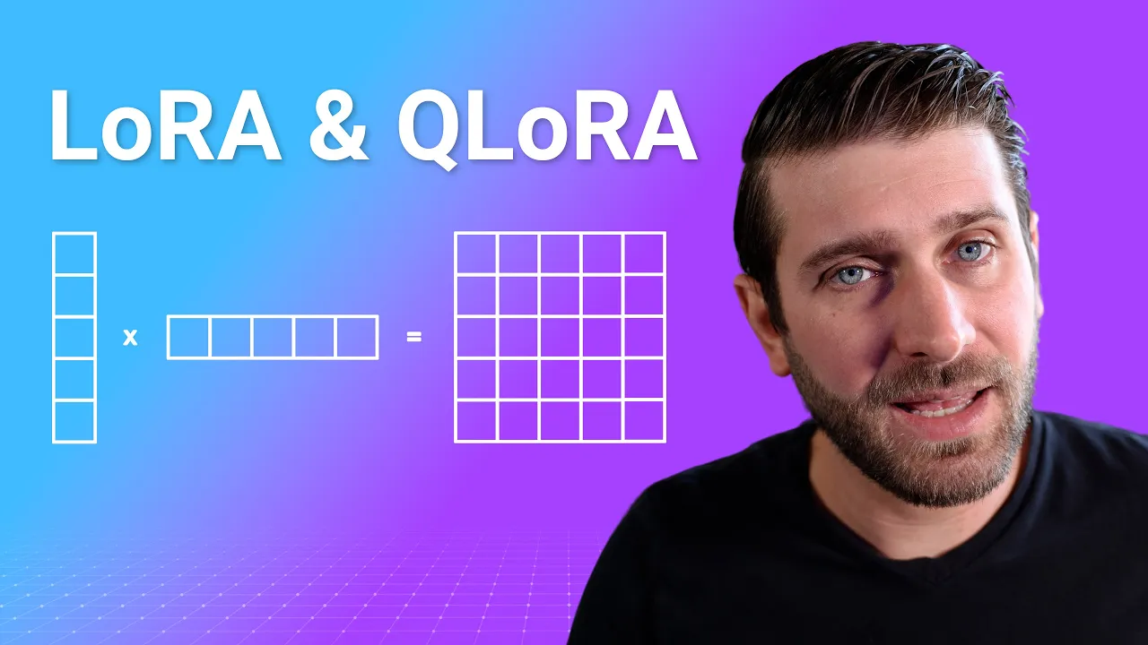
Parameter-efficient fine-tuning (PEFT) techniques like LoRA (Low Rank Adaptation) and QLoRA (Quantized LoRA) enable efficient retraining of large neural networks by freezing pre-trained model parameters and training only low-rank matrices (e.g., 6x1 and 1x6 instead of 6x6) to capture domain-specific changes, reducing computational cost from millions to thousands of trainable parameters while maintaining model performance.
How Fine-Tuning Works: LoRA & QLoRA Explained Simply
Added:Basic understanding of neural network architecture, specifically how weights, biases, and backpropagation work during training.
Familiarity with the Transformer model architecture, including self-attention and feed-forward layers.
The concept of standard (full-parameter) fine-tuning of Large Language Models and its associated computational and VRAM limitations.
Fundamental concepts of linear algebra, particularly matrix multiplication and the mathematical concept of matrix rank.
Basic knowledge of computer arithmetic representation (FP32, FP16, and INT8/INT4 precision) used in deep learning.
Practical hands-on implementation of LoRA and QLoRA using libraries like Hugging Face PEFT, BitsAndBytes, and TRL.
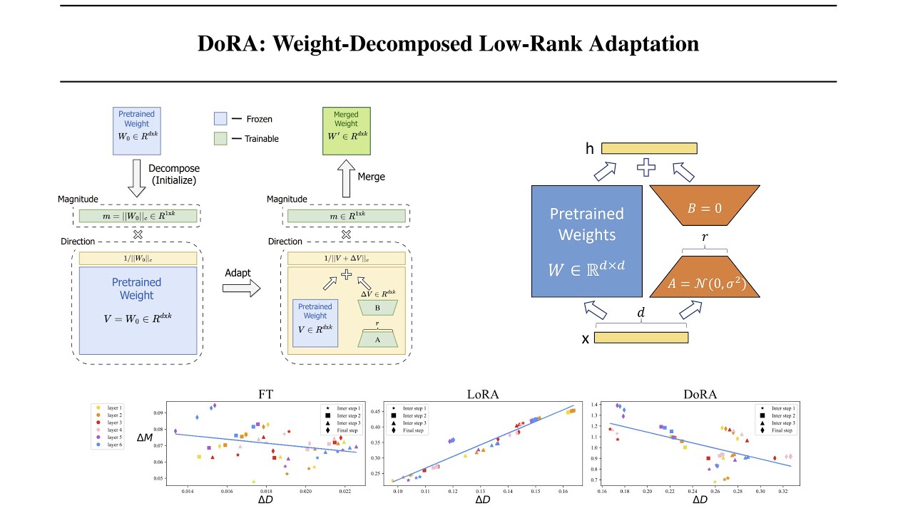
Exploring advanced Parameter-Efficient Fine-Tuning (PEFT) alternatives and variants, such as DoRA (Weight-Decomposed Low-Rank Adaptation) and AdaLoRA.
Learning the process of merging adapter weights back into the base LLM model for optimized, zero-latency inference.
Applying PEFT adapters within preference alignment techniques like Direct Preference Optimization (DPO) or Reinforcement Learning from Human Feedback (RLHF).
Strategies for serving and deploying adapter-based models efficiently in production environments using frameworks like vLLM or Ollama.
10.5K views357likes17:13Original Release: 2025-11-30
Hello Baba.
>> Hello Bach.
>> New topic.
>> Always welcome.
>> Ready. So we are going to understand a lot of basics today. Going to understand things in details. I [music] will tell you don't worry.
>> Okay.
>> So you remember I taught you a topic which is like the basics of everything like how chat chippity works.
>> Which is >> which is [music] what >> like what topic did I teach you?
>> You taught me so many topics neural networks.
>> So that is what I was talking about neural networks. Okay. So I taught you basics of neural networks, right? Right.
So you remember that there were nodes in layers like layer 1, layer two, layer three.
>> Yeah, I remember.
>> And then it had like all the nodes were connected to each other >> with some different weightages and all.
>> Correct. So how important is a particular input? We understood from the weight >> and then there were biases, right? So these weights and biases are called parameters of a model.
>> Okay.
>> Okay. So you must have heard that a model is like 12 billion parameter model or 8 billion parameter model.
>> So what happens inside is that in the end there are 12 billion weights and biases that we are trying to learn.
>> My god 12 billion.
>> Yes. Okay. So this is the basics.
>> Okay.
>> Now we also talked about one more topic which is called finetuning.
>> Yeah I remember.
>> Yeah. So why do we need fine tuning?
>> Basically to retrain the model with the latest uh inputs available.
>> Correct. Right. So like for example if you want a model to be specialized in a particular domain like medical or like law because our usual models are they are generalized models. So like software developers are also using them lawyers are also using them medical folks are also using them but now we want our models to become specialized in a particular >> particular field. Okay. Particular topic. Okay.
>> So then we do retraining of the model or fine-tuning of the model. Yes.
>> Right. So today we will talk about if the model is so huge, how does fine-tuning happen internally?
>> Okay, interesting.
>> So how does fine-tuning happen internally is the topic of this video.
>> Okay, [music] >> sounds good.
>> Very good.
>> Let's get started.
>> Definitely.
>> Before we move it, I would just like to take a minute over here to tell you how you can learn live with [music] me at ED courses. At courses, we have various courses for interview prep. I have high level system design, low-level system design, DSA. for project based learning.
If you want to create really interesting scalable projects, not simple clone ones, check out HLD. It is MER plus DevOps plus HLD. We have hands-on generative AI course where I have not just covered the application side but also the internals of LLM in a lot of detail with white paper discussions, transformer architecture and so much more. 10 hands-on projects have been covered over there. Please check out the curriculum, the testimonials, the LinkedIn profiles of our all our students is tagged. Plus, if you enroll for [clears throat] any of our courses, you get lifetime access to all the patches, the past patches, the future patches. So, you'll get access to the zoom recordings of the live class. So, you actually get a feeling that it is live itself. This is a feedback that I have gotten from all our students that it really feels like it is live only even if it is not live. But if you want to attend live only, you will get access to all our future patches as well. So, [music] at least check it out. I would love to be part of your further learning journey. And if you still have any questions, feel free to reach out to us at supporttheredcourses.com or just drop a WhatsApp or call us at this number. [music] And now let's continue. For starters, let's get started with the 10 billion parameter model.
>> 10 billion. Okay.
>> Okay. So now there are trillion parameter models also but we are taking one standard 10 billion parameter model.
Okay.
>> Okay. So now in the end these parameters are what? Weights and biases are what?
>> Numbers basically >> it's all numbers right?
>> Now it is basically decimal number.
>> Okay. Okay. And in computer everything is represented in bits by >> binaries.
>> Correct.
>> Right. So every number can be like a 32 bit number which is like four bytes.
>> Yeah.
>> Or it can be a 16 bit number.
>> Let's take 326 which is like two bytes.
>> Okay.
>> Okay. Now when we are talking about 10 billion parameters.
>> Yeah.
>> Right. So that will be how much space?
Let's just talk about storing 10 billion parameters. So every parameter let's take the smallest 16 bit for now.
>> So 10 billion into 16 bits or you can say [music] two bytes >> 116.
>> So that is 20 GB actually.
>> Yeah.
>> So 20 GB just to store the 10 billion parameters. Then another 20 GB because you remember for weights and biases what is the goal of the neural network that we have to do the training and we have to optimize and find the correct values.
>> Correct values. Right? Now to find the correct values we were doing differentiation and we were finding gradients. So weight and bias with respect to you remember we have to minimize the cost and all of that right.
So uh to store the gradients for these again we need another 20 GB and then for optimization because there are algorithms that are running for optimization. So it has like if you see like a normal optimization algorithm like a dam is a very famous algorithm that takes 100 GB for a 10 billion parameter. So if I take 20 GB to store the just the parameters >> 20 GB to store the gradients and the 100 GB for optimization related things that is 140 GB >> just for a 10 billion parameter training.
>> Oh god.
>> Okay. So do you think it is very easy to train a 10 billion parameter model? Uh I don't think >> yeah [laughter] >> definitely >> right so retraining a model is not very easy >> easy yeah >> correct >> certainly >> but we also want ways to be able to retrain and make our model very good >> understood >> correct so that is the problem right now >> and make it easier also >> yeah yeah [laughter] right so this 10 billion parameters if I decide that I want to train all the parameters again that is called full parameter finetuning >> full parameter fining >> that I'm going to train all the parameters again >> okay we discussed finetuning now it full parameter tuning all the parameters will be retrained >> correct I'm guessing now you can imagine that we don't want to retrain all the parameters >> certainly because the time computation and all of that right it I'm talking in terms of storage but also the computation the time everything right >> certainly >> so there comes parameter efficient finetuning >> okay or parameter you can call it optimization also >> yes this is called pet parameter efficient fining Okay, >> parameter efficient finetuning.
>> So basically what I maybe it's a guess work the important parameters you'll pick up and fine-tune them.
>> So we'll talk about that how to achieve PFT.
>> Okay.
>> Okay.
>> Am I correct?
>> Yes.
>> Okay.
>> To an extent. Yes.
>> Okay.
>> So I just drew this diagram. You remember this is neural network.
>> So I have now connected only two layers like this. All the nodes are connected to connect different. Yes. So every connection is going to have a weight and then there are biases. We know all >> definitely.
>> So now there were different methods that were explored for parameter efficient finetuning. Okay. One way is that what if after the entire thing we put one extra layer that we are going to use to train using the new data.
>> Okay.
>> Okay. But now see in every model now there are two phases. One is the training phase. Now after we finish the training there is the inference phase or when we are going to use the model.
>> Okay.
>> Correct?
>> Okay.
>> So what happens during the training we learn the weights and the biases. But when we use the model what happens is that we actually do the calculation. You remember y equal to m express. So once you have learned all the things all the parameters then you are just going to compute the output values for a input value. Right?
>> Definitely.
>> So that is called inference.
>> Inference basically dering deriving out of the >> the input. Right. So after training happens inference when you give an input and you'll get the output. Right? Now the thing is that if we add one extra layer okay we will be able to train and we are not going to change the rest of the parameters. So we are going to do training and learn only these extra parameters.
>> Extra parameters. Okay.
>> But now what happens is that inference time also increases because now there are so many extra parameters. Right. So that was not considered a very good solution.
>> So what better solution can be there.
Right. So this is one solution. So like this there are many solutions.
>> One solution is adding another layer.
another layer that we are not going to learn all the parameters. These will be added layer we are going to so this added layer will learn the extra things that we need to learn for this particular domain >> like that right so it will have its own weights and biases but what happens is because of this the inference also becomes slow >> slow >> right so this is one way that you can add one layer at any of these points you can add it in the end you can add somewhere so this is one way of achieving parameter efficient finetuning >> okay >> but now there is some maths involved which is very very interesting and I want to tell you that so that you understand what other ways are there the better way okay so at any particular layer there are going to be lots of weights >> you remember when I had taught you a bit about self attention I had told you that everything is represented in terms of matrix [music] >> what is the impact of every word on every other word and all that yes >> so here also when we have so many weights no they are represented in terms of matrices >> okay >> okay so it is like one layer node how is it connected to the next layer nodes so suppose m node nodes here, M nodes over here. The weight matrix will become M into M >> M into suddenly >> how how is every node connected to every other node. So every node is going to have a weight [music] >> correct.
>> Now this weight matrix it can be of 10 tens of thousands right? It can be like 1,024x 10,24 10,000 by 10,000.
>> For simplicity to just give an example, I'm taking a 6x6 weight matrix. Very simple example. Simple simple. Okay. So if we take a 6x6 matrix, how many elements are going to be there inside that?
>> 36.
>> 36, right? So 1 2 3.
>> Okay. Now there are 36 elements. Okay.
Now if there are 36 weights what we have to do is we have to see that we have to change these weights somehow right we have to when we do training what are we doing we are finding the new values of weights and biases >> yes >> correct so one way would have been that I would have updated all the 36 weights right >> but the better way will be which has more significance >> that is true >> but think about it so if I have another >> matrix >> matrix which I can call as a delta w matrix Okay, >> this is like how much do I have to change the weights for the new domain right for the specialization >> basically change in the weights >> correct change in the weights so then now the goal becomes that I don't have to touch the already weights and biases that is a pre-trained model so now weights and biases are fixed >> but the goal becomes to find this delta w >> delta w okay >> right so delta w will also be 6x6 >> 6x6 >> right now the goal is to find these 36 elements >> okay >> right Now okay now think about it. So now instead of this 6x6 matrix >> okay >> what if I take two matrices of 6x1 and 1x 6 size.
>> Okay.
>> So when I multiply these two matrices what happens >> again 36 >> 36 elements right? But if we have these six into one so how does it look like?
This is 1x 6 and this is 6x 1.
>> Yeah.
>> So how many elements are there now? Six elements over here. Six 12 elements over here.
>> But when we multiply these two how many elements do we get?
>> 36. 36. Yes.
>> So what this is the concept of matrix decomposition >> that instead of training to find 36 elements >> we are finding only 12 elements.
>> 12 elements.
>> Okay. Making the task easier.
>> Correct.
>> Simpler.
>> So now see right now we have taken the example of 6x6. But it can be 1,000 by,000.
>> Definitely.
>> Right. So if it was 1,000 by,000 we would have to learn 10^ 6 elements. But now we would have to learn only 2,000 elements.
>> 2,000. Understanding.
>> Understood. Understood. This is called low rank matrices because this is like rank is one >> one. Okay.
>> Okay. So this is called lora.
>> That is low rank matrices.
>> Low rank adaptation.
>> This is called low lower rank.
>> This is called lora. This is parameter efficient finetuning that instead of finding 36 new elements [music] now we'll be finding 12 new elements.
>> Okay. Okay.
>> Yeah.
>> Okay.
>> Yes. So this is called low rank adaptation.
>> Adaptation.
>> Just one more thing over here. Just think about it.
>> Sure.
>> Now see if I am taking 12 elements instead of 36 elements obviously efficiency somewhere will go for compromised.
>> Yeah. So it is a tradeoff right. But if we consider computation right because we are saving so much of computation like think about 10^ 6 and 2,000.
>> This trade-off is considered okay.
>> Okay. Okay.
>> But if you still want to adjust it what you could do is you could take a 6x2 and a 2x6 matrix.
>> Yeah. you are adding to it.
>> Yes. So then it would look like two rows and this and then two and this >> basically 24 elements.
>> Yes. 24 elements. So if I take 6x2 and 2x6 [music] the comput efficiency will become more but computation will also become more.
>> Yeah. It will take some time but efficiency will improve.
>> Yes. So that you can adjust using that how many rows and columns you want. This number is called rank.
>> Okay.
>> That is why low rank adaptation. [music] So if you take only one row, if you take six by one, one by six, that is rank one.
>> Low rank adaptation. This is also low rank.
>> This is also with rank two.
>> This is with rank two. Like this you can take with rank three. You you might now understand the rank will obviously be lesser than the size of the >> definitely. Definitely. Right. So [clears throat] it can be rank one, rank two, rank three, four, five, six. But as you increase your rank, the computation that you require will also be more but efficiency will also increase. Yeah.
[snorts] >> So this is called lower rank adaptation.
Okay, great.
>> So what is happening in parameter efficient finetuning that [music] in these weights and biases are frozen >> frozen >> for few layers for few important layers what we are doing is we are going to retrain for these 12 parameters or for the low rank >> 12 or 24 whatever we decide >> so low rank matrices >> low rank matrices [music] >> interesting >> definitely >> so now the last topic is that how can we make this even more efficient >> even after low rank you want to make it further efficient okay without increasing the computation.
>> Yeah. [music] Yeah. Interesting.
>> So you remember we started with that every parameter, every weight of bias in the end is a decimal number of 16 bytes or 32 bytes. 32, right?
>> Now what if I can have the same understanding or the same precision by a four bit instead of a 16 bit or instead of a 32bit.
>> Okay. So if that was possible then [music] we would just have the uh saving of by four right instead of 32 starting we are using four bit so the saving is directly by 8 times 32 and 4.
>> Oh yeah >> right 16x4 >> 1/8.
>> Yes. Okay.
>> Right. So you are going to save on lot of computation.
>> Lot of computation.
>> So this is called quantization.
>> Quantization.
>> That every parameter you are going to quantize it to four bits.
>> Okay. Right. from 16 bits or 32 bits you are quantizing it to four bits.
>> This is called Q Lora. Quantized low rank adaptation.
>> Okay.
>> Quantization is a generic concept but when you apply it with Lora over here it's called Qura.
>> Okay.
>> Okay. Now one more interesting point over here like normally people would think that when you represent the same thing in four bits obviously the precision is going to go for a toss like people do think like that right >> but there are white papers that have proven that no that is not true >> so what happens in quantization I'll tell you one very interesting thing >> sure >> have you heard have you seen this curve somewhere >> certainly >> this is a quashian curve or a bell curve like it is very common >> it's commonly used in normal theorems probability >> very good in probability and all right so what usually it says is central limit theorem if you have heard definitely right so what it says that usually the parameters like land up in this particular curve >> 99.7% will come >> correct correct correct right so the same weights and biases actually same thing applies over here and every parameter can be represented using four numbers on this curve >> okay >> so that is what four bits is used for Oh great.
>> So now instead of representing everything in 32 bits or 16 bits you represent using only four bits that are there on this curve >> on this curve.
>> Yes.
>> Okay. Great.
>> So that is how quantization is.
>> Very nice. Very interesting.
>> So this is Qura. So this is Lora Qura.
This is how fine tuning happens in here.
>> Low rank adaptation and quantization.
>> Quantized low rank adaptation.
Interesting.
>> Very interesting. So there are libraries and there are companies that are specially like you know working on this that how can we apply algorithms for Laura how can we make >> very good very interesting thank you >> did you enjoy >> certainly >> what topic should you learn next >> that you can only tell me should tell >> ah of course your audience can tell better but if you have found this interesting do like share and subscribe >> thank you >> thank you >> thumbs up for papa okay bye >> thank
Up Next

14:48
Hugging Face Transformers Library: A Beginner's Tutorial
@AssemblyAI
616.7K views•2022-04-03

57:48
Secure Multiparty Computation (MPC): Foundations & Challenges
@SimonsInstitute
7.3K views•2015-05-28

13:03
Bypassing Tor Censorship: Bridges and Pluggable Transport Guide
@Coding_ForEveryone
397 views•2024-06-11

18:41
Neural Networks Explained: Math, Layers, and Learning Fundamentals
@3blue1brown
21.9M views•2017-10-05
Related Study Plans & Knowledge Roadmaps
Structured learning paths in Artificial Intelligence
artificial-intelligence
Aligning LLMs: DPO, TRL & Custom Datasets
01Foundations of Python & Machine Learning
02Transformers and Large Language Models (LLMs)
03Aligning LLMs: SFT and RLHF
+ 3 more learning modules
24h6 modules
Explore Roadmap
artificial-intelligence
Federated Learning: PyTorch, Flower & Privacy
01Python & Machine Learning Foundations
02Deep Learning Basics with PyTorch
03Introduction to Federated Learning
+ 2 more learning modules
35h5 modules
Explore Roadmap
artificial-intelligence
Securing LLMs: Guardrails AI & NeMo Gateway
01Introduction to LLMs, Python, and APIs
02Understanding LLM Vulnerabilities & Threats
03Defending LLMs with Guardrails AI
+ 2 more learning modules
15h5 modules
Explore Roadmap
artificial-intelligence
Building Recommenders: Two-Tower & Vector DBs
01Foundations of Python & Machine Learning Basics
02Introduction to Recommender Systems
03Deep Learning & Representation Learning
+ 3 more learning modules
75h6 modules
Explore Roadmap