









![Foundations for Machine Learning | Linear Algebra, Probability, Calculus, Optimization [Lecture 1]](https://i.ytimg.com/vi_webp/C8hEa2qb46k/maxresdefault.webp)



![[Paper Review] GNN for Time Series Anomaly detection](https://i.ytimg.com/vi/n-ZDl3d7vR4/maxresdefault.jpg)





![[GNN] Graph Neural Networks. Graph Learn. Graph Neural Networks GraphRAG, Knowledge Graphs. GNN LLM](https://i.ytimg.com/vi/do1LKszfGqI/maxresdefault.jpg)

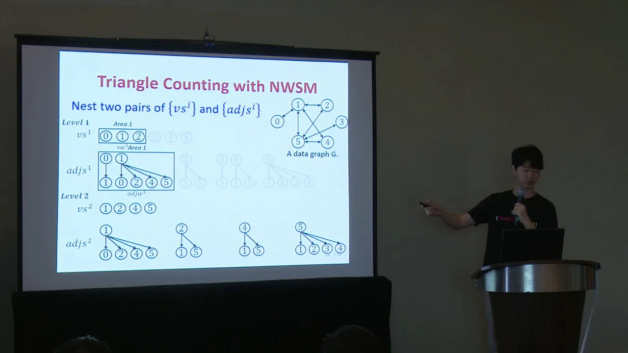





This lecture covers two primary approaches for detecting anomalies in static graphs: (1) Feature-based methods that use handcrafted features such as node-level metrics (eigenvector centrality, betweenness, clustering coefficient), dyadic features (reciprocity, common neighbors, Adamic-Adar index), ego-network properties, and global network properties, which are fed into classifiers to identify anomalous nodes or edges; and (2) Pattern-matching approaches like ODDBALL that define specific types of anomalies (near-cliques, near-stars, heavy vicinities, dominant links) and use feature dependencies (number of nodes vs. edges, total weight vs. edges, principal eigenvalue vs. total weight) to detect deviations from normal patterns in ego-networks.
Anomaly Detection in Networks | SNA Lecture Part 2
Added:all right so today we will uh continue with this chapter called uh animal detection graph anomaly detection and last day we have discussed about you know the motivations behind annual detection why this is an important problem why it is a difficult problem we have discussed many uh issues right that people generally face for uh to to address this problem right now now let us look at some of the methods right i will not go to ah go into each and every details of this method there are plenty of papers on graph analytic detection but i will touch upon some of the methods and i will briefly talk about some of them and i will uh explain you know in details some of the methods that are that's a very important okay so if you look at the overall taxonomy this is the taxonomy of graph analytic detection so we have static graphs we have dynamic graphs now static graph we look at you know plane graphs and attributed graphs right plane graphs uh nodes or edges do not have attributes attributed graphs nodes and edges have attributes and then we look at two types of methods one types of method one type of methods purely depends on the structural property of the network right for example a star looking at the star type of subgraph or a click type of subgraph or you know or some edges which are highly you know connected and so on and so forth whereas in attributed um what is in community based uh approach right we look at you know at anomaly anomalous nodes with respect to a particular community right so graph based graph based anomaly detection there are two different you know approaches one looks at the one approach looks at one one of course tries to identify anomalous nodes anomalous entities from the entire graph another approach looks at the communities right clusters and then try to identify then tries to identify uh entities within the cluster which seem to be anonymous right so these are more of a local type of approach because uh these anomalous nodes uh are marked as anomalous with respect to particular community when when you look at the entire network structure those nodes may not be anonymous right but when you look at a particular community uh it may look like a like anomalous like an anomalous mode or entity for example say ah for example say um you know there is a uh so there's a lab right uh there's a research lab uh there are uh there are 15 members in the research lab and uh say 13 members are doing phd two members are doing masters right so these two members are basically anonymous members with respect to that community with respect to the lab but if you look at the overall say scholarly network right nodes are researchers and links or connections some connections you look at different labs right and uh so this master students right they are not anomalous knowns because in the network there are so many anomalers so many master students right but with respect to that particular uh community for the particular cluster those nodes are anomalous right and then we we look at some of the relational learning based approach where people basically try to look at the relations between entities and try to reason out that okay this this relation is not uh this relation should not be there between two nodes right because because these these two nodes uh belong to the different types but you know but this particular relation exists between these two nodes so therefore uh this relation is a this particular these two nodes are anomalous nodes or the link is an anomalous link right we look at some of the approaches there uh in case of dynamic graph uh we mostly look at the plane graph here dynamic graph meaning uh here graph structure changes over time topological structure changes over time so you know we mostly look at the plane graphs we will not look at the attribute attributed dynamic graphs so here we assume that you know the network structure changes over time so we have snapshots of the networks at every time right at p1 you have the native snapshot at t2 you have snapshot t3 of the snapshot and then you look at uh you know topological difference uh topological differences across two time stamps so at t one then at a t and then at t plus one right you look at the topological structure and you see whether they are different or not similarly at t plus one and t plus two you look at the topological difference and then you decide right and so on and so forth so you decide across every consecutive time stamps and then you take some aggregated approach and you decide that okay this snapshot or or or these two nodes right or these sub graphs uh are anomalous subgroups okay so i will talk about one such approach on annual direction for dynamic graphs okay so let's start with the static graph the idea is very simple so the given the the input is that you have a snapshot of the graph right meaning so there is no temporal information available you have a static network right and the task is to identify nodes or edges uh or substructures right which are analogous which appear you know which look very different from the remaining part of the network okay and we look at plane graph and attributed okay so let's look let's first start with the static approach for plane graph uh sorry the the structure based approach for plane craft okay so so if you look at the older papers right paper published in 2009 2010 they mostly relied on handcrafted features right and then some sort of classifiers to classify nodes or edges based on those features right and those handcrafted features are very carefully curated and for that you you may need to know the the the domain in general for example say you want to detect anomalous transactions right for transactions so you should be you should know the underlying you know dynamics the underlying um setting when a transaction happens what are the important factors behind the transaction and so on based on that you can curate the features right and i'm talking about uh methods uh you know pre-deep learning and i think about it right 2009 2010 during that time even before that 2005.56 during that time okay and uh people also looked at different proximity based so so this kind of approaches mostly deal with features so you extract features different types of features for example you know some node centric features like centralities right clustering coefficient and so on degree and so on and then you you know you employ some classifiers in classified second approach you look you you design some sort of proximity based approach right it basically says that you know you have nodes and you also know the proximity between numbers and let's assume that you have the liberty to measure the proximity of all pairs of nodes right so you have nc2 pairs and then you uh you basically measure the proximity and then you flank those pairs of nodes whose proximities are very very different from the other proximity but it is also important that you know those two nodes uh those pair of pair those pairs of nodes should not be very far from each other because if they are very far from each other automatically their proximity will reduce but that doesn't mean that those nodes are anomalous nodes will talk about okay so feature based approach okay so people generally took into account these five sets of features okay so the first set of features called node level features where people look at eigen vector centrality closeness centrality between the centrality and this is node centric analytic mutation you have a node and you did it whether this is anomalous or not between a centrality local clustering coefficient and degree associativity all these you know matrix we discussed in the previous lectures right uh node centric features are important we also look at something called dyadic features static features basically those features which can be curated by taking into account the pair of nodes so you have a pair of nodes and then you extract some features for example there is something called reciprocity we discussed right there is something called uh you know reciprocity basically says that if if if a follows b whether b follows a or not so it's a it's a property of a pair of nodes not a dyadic property right similarly age between us because age ultimately connects two nodes so whatever feature that you extract uh you know for a particular age right so those all all those features are essentially uh dyadic features because the those features essentially take take into account two nodes right so age between your centrality is a dyadic feature number of common neighbors you take two nodes and then look at the kind of jacket similarity atomic distance i hope you remember we discussed uh in the link prediction chapter there's something called adamic adder right which essentially looks at the commonality between uh you know pairs of nodes community of commonality between neighbors for a pair of uh for a pair of nodes and then you get some number right and you then you you then for each for each such common neighbor you take one by log of uh the degree of that one right you discussed last class in the link prediction chapter uh of course you can think of many other properties here many other features here egonate so egocentric network is a very important uh structure that we consider in case of anomaly detection what is igonet i hope i have already discussed but let me quickly tell you what is egonet so ego net is essentially you know let's let's see let's assume that this is your graph right this is your graph um right and this is you so ego net is a small network of a particular node right so if you if you uh if you extract the ego network for this for node u so what you need to take into account you need to take into account uh the particular node that node and it's one of neighbors it's one of neighbors and their connections right so you basically take this node this node this node this node this node and this node and their connections right so ego network of a node is essentially an inducer graph of that particular node and its neighbors and its first degree neighbors first of all right so the ego network of node u would be this right would look like this okay this is the ego network so this is called ego right the central node is called ego and this is called the alter so these are alters the one of neighbors are called orders so for every node we have such a good network now in this ego network you can extract different properties because ultimately this is also subnet right you can extract number of triangles because number of triangles will give you ideas about the clustering coefficient right so number of triangles total weight of the ego network right uh total weights of ages of the ego network then uh principal eigenvector of the adjacency matrix of this ego network and so on okay of course you can extract many other features maybe many other ignite centric features uh node group uh you can look at a subset of nodes right it may not be gone but but say a selected subset of nodes say you can say that i i want to look at you know nodes within two hops so first top and second one and then you construct the network right then you can extract uh density you can extract modularity right you can extract conductance so this density modulated conductance these are also network centric properties right because modularity ultimately measures the community uh you know community likelihood or whatever right whether the network possesses a community or not conduct is also a network centric property but all the intercentric properties can also be measured for a particular group of nodes right ah then we have global properties for example total number of connected components right in the graph then distribution of the size of the you know different components then you can take know um some shortest path you can take average degree global clustering coefficient and so on and so forth so these are all network synthetics okay so these features can be fed into classifiers uh for and then you have you can use standard classifiers for classifying nodes and analysis or not okay uh the first pioneering paper the first pioneering attempt uh was this one which is called oddball right oddball is a very interesting algorithm not an algorithm this is more of a pattern matching kind of approach where uh you you decide a particular type of anomaly that you want to detect and then you start looking at some of the patterns those you can use for detecting those types of angles right for example you say that look i i want to identify all stars because i know that in this graph if there is a star that's an anomaly okay so then you can devise an algorithm to detect all the stars right so so so this is the idea so you you uh define your own definition you you define anomalous nodes right the types of anomalous nodes and then you come up with ah features which you can use for identifying those anomalous nodes right now this is different from the feature based approach that i mentioned earlier although this is also feature-based approach but the previous approach was basically you know you curate you curate a set of features then you let the classifier identify which features are important which are not okay so uh right so so this oddball they are interested in these three types of anomalous ah anomalous nodes right or animal substructures right so the first anomalous of structure is something called near click or near star these are two structures though so near clicks are those which which are clicks but not a completely granted graph right but but say if you have 95 percent or 98 percentages present in that in that graph in the subgraph you can say that okay this is a this is an anomaly right so near click and near star near star as you can also understand right not a complete start like this okay but most of the edges exist okay so this type of these types of uh anomalous structures they wanted to identify the second one was something called heavy vicinities so the idea is that and and this particular definition was adapted uh for a particular type of network right and this is this is who calls whom network so uh individual one uh one individual is calling another individual or you can connect uh an edge between them and the number of calls between two individuals within a particular duration that would define the weight of the age right so i'm just reading this thing forwarding so what it is saying that if person if person i has you know contacted any distinct person in distinct people in a who calls home network we would expect that the number of phone calls so number of phone calls uh for a particular pair of nodes would be the weights of the dates right would be a function of of the n right so basically you know n is a total number of um nodes present right and and if if uh you know if this is normal then you can think of you know the age weight would be approximately uh you know uh asymptotically order opinion not more than that right extreme total weight for a for a given number of contacts in would be suspicious right for example you look at this one right okay so this is this is the uh the node and these are all the callers who this particular node has called okay and you see the weights right so all the edges most of the edges are you know very um less weighted meaning that the those edges are kind of you know normal edges but if you look at these ages right these edges the weights are strong right waist weights are heavy so this is this is uh and and if you look at the uh the corresponding eo network you may you may be able to get this kind of big one right where you remove some of the edges with less weights and you get this kind of ego network okay uh the last one is called dominant uh you know heavy links so here again the idea is same so the idea is that you know again think of this who calls home network now if there is if there are one or two such edges with extremely high weights right with extremely high weights for example in this case you see this age has extremely high word you can say that okay you know this is definitely an anomalous behavior now this kind of you know who calls whom network this kind of things happens in many ways for example you know there is say for example there is some some some noise or some error in the in the um in the in the in the dialing pad right or in the dialing system right so automatically you know uh you your your phone without your intervention right your your phone is your phone calls another phone right because of the dialing problem right so these kind of animals are important to detect for telephonic mostly in the telecommunication networks okay so so this four types of patterns clicks starts heavy vicinities and dominant you know heavy links these are the patterns that this guy oddball this paper wanted to detect okay so now let's look at what are the features that they have tried out they have tried out multiple features by the way right but these four features seem to be useful to detect these anomalies right so the first one is the number of neighbors of an uh of an ego eye basically num basically the degree of that ego i right and that egocentric network you just look at the degree that is a9 right so what you do here you first extract igo nets of all the nodes you take a node you extract the ego net and you analyze right so the pro the properties or the metrics that i am going to discuss now those are calculated for individual uh ego network okay so number of neighbors number of ages indigo network right but remember number of neighbors and number of edges are different why because within the uh alters within the neighbor there might be edges and that would be that would be counted within ei but that that would not be counted in a right what is w y w is the total weight of the equivalent so basically you take the sum of all the weights of the edges present in the unit and this lambda lambda you know w i this is the principal eigen value uh of the weighted agency matrix of the ebony time so you have the network ego network structure you get the adjacency matrix right weighted okay then you do an eigen decomposition uh sorry eigen value eigen vector calculation and you extract you identify principle ah largest eigenvalue and the corresponding principle again right so that principle eigen value could be used as as another proxy for detecting this okay then they looked at all combinations right and what they concluded that when they drew the graph of number of edges and number of nodes right x axis is number of ah edges and y x is number of nodes right whatever vice versa if these two features are comparatively used right if you look at the growth of e with respect to n a growth of n with respect to e and so on this should be able to identify the clique structure and the star structure okay if you look at the w and e w is a total weight and e is the number of pages and if you look at the if you study the comparative again the kind of competitive study or the dependency between w and e right that would help you identify heavy vicinity okay and the third one if you are able to identify the principle eigen value and the weight and the total weight of the ego network it would give you a hint to identify the dominant pair i mean the the last category that i mentioned the dominant age pair right i mean the the dominant pair of nodes so the the dominant edges okay so they tried with different combinations different compositions different dependencies but these dependencies turned out to be useful again in an unsupervised manner these are all unsupervised approaches right to identify cliques stars heavy vicinity and dominant pairs okay then let's let's look at some of the results so so this one uh let's first look at the you know clicks and stars okay and this is little bit difficult to understand therefore i am suggesting you to only focus on one graph the other graphs will be automatically understood let's only focus on this this graph okay this plot so what they suggest is that so their first observation was that the number of nodes and the number of edges in an ego network follow a parallel property meaning the change of the edges is proportional to the power of number of nodes you see e i is proportional to n i to the power alpha where alpha should range they said that alpha should bridge between one and two now if uh if an ego network follows this property then this is normal then the ego network is normal if it doesn't follow then there is some problem okay or or ah you know or or if if we see that certain ego networks are very very different from other ego networks then there may also be some problems okay so let us look at you know this plot so this is on a data set called enron data set there are three data sets postnate enron and oregon so we first look at the enron data set okay and i'm drawing it so x axis is the number of nodes which is ni and y axis is e i number of pages right so you identify an igonet and you identify nii similarly you identify another igonet and you determine eini so you have you have n number of such pairs in i e i n i e i for every ego net you have a pair in iei value right so what you do you right and how many units are there there are in number of big units because each ignite corresponds to a node right so number of nodes equal to number of equivalents then you plot a dot so this one dot correspond to an ego net right for example this is the dot so the x axis would be the corresponding a9 and the y axis with corresponding ei similarly you plot all the dots so this is basically scatter plot okay okay and then what you do so this is scatter plot okay then what you do then for every ni right not for every ni you can choose sum in i for example 10 100 right thousand and so on uh when ni is 10 you have many points right you take the median you measure the median value median ei similarly when ni equals to 100 you have many points you you you take median ei similarly for when ni equals 1000 you take the median value because you have many points here you take the media right and so on and so forth so you get the median value you could have also taken average what they took median values okay median has certain certain advantages okay and then you feed a linear line you can easily fit a linear line using say some least square error feed or whatever right you fit a linear line right and you also know that if e i is proportional to in i and if e i is proportional to n i square how would this graph look like right so e i equals to n i may look like this right or some something like this right so say this is ei equals to ni and say this is ei equals to ni this is when alpha equals to 2 and this is alpha equals to 1 this is the bound right this is the bound and now you may see that's how the data points which lie this points or in fact below these points above these points right meaning these these ego networks right are very very different from the median value right and that it it they do not follow this range which is this one and then you identify these points i mean this ego network and corresponding nodes as uh anomalous as as anomalous terms right so this is a plot you see here right this blue line is uh power law when alpha equals to two this is when alpha goes to 1 this red line is um is the media is the linear fit right all these black dots are median values and green line green points are basically points corresponding to all the ego networks okay okay and then then you look at some of the points which are very different from for example they looked at this point they looked at this point right and they manually identified those points so interestingly some of those points are very different because say this point correspond to some co so this point corresponds to the ceo of enron can lay right and of course in a in an enron graph right you have other callers and ceo's calling pattern might be very different okay similarly they did the same experiment for these data sets and if they found these points and these points as anomalous nodes right in these data sets they found these points and anomalous nodes and they they tried to justify that look they are actually anomalous because they are uh either some big guys right or you know some fraudulent users and so on and so forth they then studied those data points separately okay and they said that these points right they are either clicks or stars near clicks or near stars right so then they concluded that number of nodes and number of pages might be useful to differentiate two to identify near clicks and near stars okay same thing for the other types of anomalous behavior right at this time they they look at you know heavy visibility right and for heavy vicinity they relied on two other uh matrix one is the total weight w and other is the number of pages similarly for every ego net structure you measure i sorry you measure e and you also measure w right and then you um you basically plot those points these green points correspond to those ego networks and then you know you you have a feet right and and this time they said that you know this is the normal behavior so w i should follow a power law right where uh where where w i is proportional to e i to the power beta beta is always greater than equals to 1 right and the third observation was similarly you can write but but this is for determining or identifying dominant pair right and then they looked at uh principal eigen value and the total weights right so uh for every ego network divide you first uh you first draw the adjacency matrix mutation matrix you determine the this one primary uh principle i can wear eigen value largest eigen value and then you plot this this against the total weight and then you do the same thing fit and look at abnormal points okay this is the you know approach of a simple feature based approach you look at the features and you consumer waste where you do it you detect it in an unsupervised map okay okay so now we look at some of the you know approaches uh these these approaches belong to proximity based approach where look at proximities between nodes and then we determine the anomalous behavior right so here you can use different types of features for example page rank random work with restart personalized page rank sim rank right or its variations all these things we discussed in the link analysis chapter we can use simple jacket proximity and any any any you know any types of metrics that we generally use for link predictions right so the idea is here is that you know uh you you use these proximity based features and then if if you see that okay you know uh a personalized page rank for example is very very different from these methods are very i would say very ad hoc because these are proposed long time back and you know people were satisfied because those methods actually work in reality right so you have you you first major page random work with these charts and these kind of approaches and then then you have thresholds for every metric and you then select those nodes which uh which basically you know lie uh above the this world or beyond beyond us as well depending upon the situation okay i will discuss one such approaches later right but uh let's let's wait so now let's look at community centric method so here the idea is that we first identify a community there are two ways to to attack this problem the first way is that you first identify the community using some community detection algorithm and then you dig deeper into the community you identify some anomalous notes that's the first chapter second approach is that you identify community and anomalous nodes jointly okay you some ways to identify communities you have similar ways to identify anova last notes you you essentially you know come up with such methods which jointly identify uh identifies both communities and outliers okay how do you do that so so in this paper this sun at all paper uh they mostly relied on bipartite network right so they used publication network right author versus paper or peer peer-to-peer p2p network right or some financial trading network customer product network and so on so here the problems are how to found how to find a community of a given graph which is also referred as the neighborhood of a node now there is a little difference between the community that that they are referring to here and the community that we discussed in the previous chapter okay so here what they meant to say is that communities are those nodes which are their neighbors which are the neighbor of a node it can be one hop it can be two hours right in fact we will not take into account all the first of neighbors will not take into account all the second operators can you come up with some some ways to identify the neighborhood of a node and then how to quantify the label label of the given node to be a bridge node so they they are interested in identifying bridge nodes and bridge nodes are those nodes as we all know bridge nodes are those nodes which basically connect two communities right so they wanted to identify these bridges in some ways according to them this bridge nodes are anomalous nodes okay and how do you do that so they they came up with a very simple approach very very simple approach so they said that you know think of it right so you you let's assume that the graph has some community structure okay it's not a random graph it has a community structure but you do not know the community structure at all of course right so if you do random work with restart right if you do random work with restart based uh page rank right say personalized page rank or whatever right random mortgage with research is basically a a variation of personalized page time right because in personalized page rank you uh you said that the jumping probability right uh you basically move to a set of nodes in case of normal personalized page rank and in random work with restart you basically uh the that state is fixed the set is basically one so there is only one node right to to whom you basically jump right from the neighbor so if you have this kind of setting right this kind of setup you can calculate personalized page rank or random with listed think of those nodes right think of those nodes which are um right which are ah central nodes of a community and those nodes which are peripheral nodes of recovery now if you start personalized page rank right uh from a central node of a community right you see that you know uh uh so so so what you do uh you take a note right you do some personalized page rank you you you do random mobile restart and basically use uh those neighbors right uh through which is restart this this random walk actually moved right or passed through those nodes as the neighbors right so you start from here you do random work with restart right and you it is basically kind of a sampling approach you sample uh the neighbors right so if nodes are present within the central part of the community right so let now let's take let's take two types of nodes central types central nodes and peripheral nodes central nodes you will see that after random mobility starts their neighbors are kind of same which is very obvious because they are the center of the community and when you do random work with restart you you basically end up sampling same types of nodes whereas if you look at the peripheral nodes right and you do random work with restart you will see that you know the neighborhoods the neighborhood set is very very different from the neighborhood state of the central universe right for example if you if you do random opposition from here you would sample this node this node right and this for example along with some other nodes internally right but you will also sample these modes so this node if you only look at the neighborhood structure based on the neighborhood structure you can easily say that this is this is outlayer okay so by the time community they basically meant to say that you know those nodes which you encounter uh during a random walk with registered kind of setting okay and then they simply said that look uh you know those nodes which whose neighborhood set neighboring set is very different from the remaining uh from from the same of the remaining nodes you just identify them as uh you know anovalus nodes and they're basically their task was to detect these nodes of course you can say that why do we need this we can even do uh you know uh some sort of between a centrality kind of approach right to identify these nodes and so on that you can do but um random walk with restart is uh is is easy uh you know compared to between a centrality or closeness centrality because these are those the centrality between the centralities need to be measured you you basically need to look at you know all possible paths and so on and so forth right or or say a distance from one node to another node now these are time taken process right but this can be used this personalized page rank this can be used as a proxy for that okay uh and then there are other types of algorithms again people something sometimes used um you know minimum description length right entropy based approach the kind of info map type approach that we suggested we did earlier for community detection right and then then you say that okay you know i i i essentially encode nodes in such a way that anomalous nodes will have high uh minimum high description length higher description length compared to the uh compared to the same for the uh normal levels right and and and this algorithm in auto part by chakraborty in in 2004 now this was again on the interesting papers we looked at information theory approach random walk with restart and then minimum description length to identify um when anomalous knows right okay now moving to the next part which is uh the attributed graph okay so so uh in the static attributed graph right we assume that we have the attributes we have attributes corresponding to nodes and then we look at those nodes which are which not only are different from the other nodes in terms of structure but also attributes right but this is also community centric right so there are many problems uh that that we encounter right but but now let me directly move to this this algorithm so this is called focus co focus focus co okay what is this algorithm saying so this algorithm is developed on an attribute graph attributed graph you see that every node is associated with a feature right and what are the features here you see that you have a degree right phd or whatever uh ms right degree is educational degree of the node you have some you know some location right you have um citizenship dutch english italian and your uh industry your affiliation right msr google etc okay and these are the this attributes are given right what is the task so remember this is also community based approach for an attributed graph the task is to identify a node which acts as a community which acts as an anomaly with respect to a community right and this anomaly is defined not only based on structure or not based on structure but based on the attributes okay for example say say let us assume that you somehow identified that this is a community okay and you see the attributes you see that you know most of them are phds only this one is a college guy college student most of them have most of them belong to new york city okay you can also say that you know there are anomalies in terms of say you know job right for example these two guys belong to bank but these two guys are part of an industry right this is industry they can be animals what the algorithm says is that we first i mean the the annotator or whatever the the third party right they they would identify they would first mention that i would like to detect anomalous nodes of a from a community with respect to a particular attribute okay and this is called this attribute is called focus attributes so what we do we first identify you know uh the subset of attributes of a particular node which are focus attributes right then we find clusters of densely connected nodes in the graph that also agree on this particular attribute right so what you do you identify the focus attributes you do not know the community structure you only know the graph right you identify the attributes then you try to i try to detect communities with respect to those attributes for example this is a community this is a community with respect to the focus attribute you know the affiliation sorry degree this is a community uh with respect to the focus attribute affiliation right or say this is the community uh with respect to the focus attributes uh you know academic degree and current location okay so you identify clusters based on focus attributes and then within the within a particular cluster you look at entities entity or entities which are different from other entities okay so an outlier is defined as a node which belongs to a cluster structurally but deviates from it in the focused attributes so you see that in this particular cluster right this node has kind of same structure as this node and this one kind of a click right but this is actually this is anomalous with respect to this attribute okay now how do you do that okay so what is the problem let's look at the input output so given a large graph g v e f number of nodes number of pages and features right and the set of exampler nodes this is very important this exemplar nodes c e x of a user use interest now say i am the content moderator or i am the administrator right i say that look in this node in this particular network these five nodes i know that these five nodes are similar nodes or these 10 nodes have same attributes that i know they are similar you do not need to identify them you do not need to investigate them i know that these nodes are similar nodes and these nodes are called exampler nodes right and let le and what would be your task your task would be to look at uh you know other nodes which are similar to exemplar nodes or which are different from examples i am given the set of nodes i am given a very small set of nodes which are same which are which are similar in terms of attributes that is given okay so what is the task what is our task our task would be to identify the weights of the attributes there are certain features what this algorithm will do this algorithm will identify will automatically infer the weight of every feature okay then what what it extracts it extracts the focus clusters that are dense in the graph coherent in heavy focused attribute so then once we identify weights of attributes then our task would be to identify clusters right with respect to the focus of with respect to the focus attributes okay and then then we look at every cluster and then we identify outlets this is the task so three major components inferring attribute weights extracting focus clusters and then detecting outliers okay so let's look at them one by one so there are some pseudo codes that i will discuss but these are not that difficult okay just just follow me what i'm saying so you are given a set of example or notes cex so these nodes are similar to each other you know that and your task would be to identify the weights of the feature uh the the weight of the features right so this beta is an is a is a is a feature weight vector okay beta one beta two beta three dot dot dot so beta one corresponds to the uh feature of the first attribute sorry the weight of the first attribute beta 2 is the weight of the second attribute and so on okay this is your task your task is to determine the weights of the attributes so let's take two sets ps and pd is for similarity d for d stands for difference and s stands for similarity so p s is a set where i will keep adding similar nodes and p d is a set where i keep adding d similar nodes so p s p s is a set where so p s would be say for example u comma v where right w comma x so on and so forth where these pairs are similar whereas so so it is basically a set of sets whatever a set of pairs similarly p d is also a set of pairs set of pairs of nodes which are different set of pairs of nodes which are similar we will populate this ps and pd okay right so now we already know that cx is a set where all nodes are similar right so those nodes can easily qualify for ps so c e x we know that c e x all nodes are similar so let's take one node from c e x and another node from c its u and v right and you can easily you can easily uh add uv pair now for every uv present in cx you pair them you pair up and you add them in ps right so now ps constitutes small cex c2 pairs these are similar pairs now let's look at these similar pairs right so for dissimilar pairs again the idea is very simple the uh for uh you know for dissimilar pairs they they they look at one node they look at they identify randomly sample one node from v minus c x set so v is the total node a c e x is a set of example nodes so the remaining nodes remaining nodes remember remaining nodes might be similar might be different we do not know we only know that cx nodes are similar we do not know what's the nature of the remaining nodes right so we sample one node from e uh from we we basically sample two nodes u and v from this set u minus c e x right and then you keep you basically add those pairs to p d now in this pairs there there are some pairs in this particular set there are pairs which might be same there are pairs which might be different right and how many such sampling happen you basically sample right this many times so ps is the size the mod ps is the size of the similarity set that we have already identified and d is the number d is what d is the size of the feature if there are five features right if say mod ps is 100 right um right and and and and mod if is five right so d is mod if so the so we we basically do this sampling right uh for 5 into 100 uh times 500 times so 500 times you choose one pair you basically you choose a pair of nodes from you know v minus cx and you add them in pd right so you see this now the set the so the size of pd is 500 and the size of ps is 100 so in balance what you do then you then then basically over sample ps over sample from ps such that ps equals to pd the size of the ps goes to size of pt okay so now you have two sets similarity sets dissimilar sets uh sorry similar sets and unknown sets right and then you what you do you um optimize this function what is this this is called mohan always distance the molar knowledge distance is one of the distance measures between two uh distributions generally okay so what it tries to do let's let's look at this function of this this objective function carefully so you take a pair i j from ps so remember ps has pairs which are similar okay and what is if i if i is a feature of node i if j is a feature of node c and what is the task the task is to minimize to minimize the distance the feature distance between these pairs of nodes because we know that these pairs of nodes are similar okay you see a phi minus f i minus ah f i minus f j right transpose a f i minus m this is the more resistance function right and what is a a is something that you want to identify right so at the end of the day i would like to come up with an a right whose diagonal elements would give you the feature importance now what's the size of this matrix this is d cross d right and these diagonal elements elements are something that we are learning so we want we want to minimize this function with respect to a okay such that right we want to minimize the entire function so the first part corresponds to node pairs which are similar the second parts corresponds to node pairs which are decimal pd now it may be dissimilar maybe not right but we we assume that most of them are dissimilar nodes so therefore minus right so if you minimize this if you minimize this it will it will automatically be maximized because minus and you see the same formula the same formula here what's the difference difference is that here i take a square root here i did not take i take a log right y log y square loop because i wanted to minimize the effect of this component why because i did not know i am not sure whether the entity is present in pd whether they are all different but most of them are different i know therefore i wanted to minimize the effect of this component in the entire objective function so therefore i took the square root i took the log okay and then i also have a gamma function a parameter right which i have control on now i i minimize it right you see that if this is an optimization problem and i minimize it and this is convex right i minimize it and i get a so a a is a matrix whose diagonal elements will be the importance of features okay one one two two so one one corresponds to the importance of feature one two two corresponds to the importance of feature two and so on and so forth so beta would be a feature vector for containing all the attributes in the diagonal elements of a sorry containing all the elements of the matrix a so what i got after this step i got the importance of features importance of attributes present in the feature set okay now what's the next task the next task is something called core identification okay so what does it do i'm not going the details of the entire thing you can read the paper right but what it is trying to do is that you know uh you so so so you see here the input is the attributed graph and the example are node right and you also have the input of a input input beta so you call this function uh in for attribute weight which is this one right and you get beta value right and then based on this beta what you do now you give weightage of every edge you re weigh the you you basically re-weigh every edge okay and this weighting is done based on the based on the attribute similarity so you already know that these two nodes are connected but you did not know the edge weight you did not do the edge weight because this is this was not an weighted graph right what you do now for every edge for every age you measure the age weight w right and this age where you see that edge weight is the inverse of the you know the similarity of uh two nodes right so higher the weight higher the similarity between nodes higher the weight higher the distinctive between nodes right of course you can do you can do the other way down higher the weight higher the similarity of the nodes is same right and then what you do you identify your threshold w dash now this w test you can extract you can identify w dash in many ways you can identify w dash from a distribution for example right you say since you know all these weights you plot a distribution and you see some sweet spot and that's your w dash right so once you identify w dash you only keep all those edges whose weights are above this w glass right so you then what you do you create another graph another induced sub graph write v s e d as f right where you only keep those edges whose weights are greater than w dash so some nodes will be removed some edges will be removed clear okay so you get a graph you create a connected component right and that's and this kind of component is something that that we call as a code set okay so then this this connected component right is fed into this algorithm now this is the main algorithm focused cluster and outlier detection right you see here find core set meaning this procedure is invoked right and you get the code ok so so here what i actually forgot to mention is that in this graph now this graph so so once you filter out all the edges whose weights are greater than less than w dash right you may end up getting a graph a sub graph which are disconnected of course right some images will be removed in between there are some images here some images here so you you will only have a graph graph but that may be disconnected okay so what what this algorithm returns this algorithm returns the different connected components present in that inducer graph say you have five counted components these five kind of components are cores right so in this course see this is a set so this course has different connected components and these content components are those components where within a virginia country component nodes are highly similar based on the features right based on the features and then what you do then the this this process is very tedious right what what basically they do they they try to explain now now you take one content component you have many connected components you take first control component okay you try to expand it you try to expand it you and to to check whether other nodes present in the graph whether they are qualified to be added to the kinetic component or not because this was a very very very strict uh you know measure that that you have taken you might have missed some of the nodes from the node switch which may be qualified to be part of the standard components right kind of a greedy let's assume that right now when you do greedy you may end up missing some points which may be qualified in later point in time for example not right now but later point in time so you take a core okay you expand the core by by looking at the neighbors right you you take a grinder component you look at the neighbors and you take one neighbor and add into that code right and you measure conductance conductance is a metric like modularity you add this neighbor and see if after addition the conduction will reduce or not remember conductance the lower the value the better the commodity structure okay so you you basically add the node and check the conduct inside if the conductance reduces then you add this node you keep on adding nodes right you keep on expanding the uh the the the content component the core right so once you add some nodes you again do the similar thing you keep on deleting nodes uh one by one and check whether whether conductance again reduces or not because it may happen that a node that you have added earlier should have been deleted okay since this is greedy i'm telling you since this is greedy you have to do all these things repeated times right so you will see that there are two protocols invited in both one is expand other is contract through expansion you are adding nodes one by one to a connected component and checking whether those nodes are also qualified to be a part of this component or not once you did once you were done when you see that okay now the conductance is increasing then you stop then again you start removing nodes one by one and check whether conductance further decreases or not if it will not decrease then you stop and that's your that's that's your final connected component final code right while doing so if you see some nodes which has been removed which have been removed right from this port right that's the outlet with respect to that core similarly you take another core because remember in uh in the course this course set right you have multiple such content components and we assume that each content component is a cluster okay so you allow the cluster to grow you allow the cluster to measure growing expanding going uh expanding contracting right and so on and so forth right and you stop when you see there is no further chance of improvement and whatever nodes which have been removed through this process those are outliers with respect to that cluster right so those nodes those nodes are outliers with respect to this cluster similarly you take another ah core right expand contract and you do that this is the idea okay this is the idea you see this is this is this contraction mechanism you see this conductance is this conductance value is measured if the conductance conductance is improving then you add it otherwise you do not add right as you see if this is improving then remove if it is not improving means if it is increasing then you remove if it is not increasing then you do not remove right similarly expansion and these techniques to me these are very ad hoc because you can also have your systematic way to do this thing but the idea is very interesting okay
Up Next

Graph Analytics and ML for Fraud Detection Using TigerGraph
@TigerGraph
308 views•2020-11-04

Introduction to Secure Multiparty Computation with Yehuda Lindell
@fhe_org
7.7K views•2021-02-04

HTTP Requests Explained: GET, POST, PUT, DELETE
@codecademy
103.1K views•2021-10-07

Enigma Machine Mechanics: WWII Encryption Explained
@JaredOwen
13.2M views•2021-12-11
Related Study Plans & Knowledge Roadmaps
Structured learning paths in Computer Science