











Q-learning is a model-free, off-policy reinforcement learning algorithm that learns the optimal policy by iteratively updating a Q-table using the Bellman equation and temporal difference error, where the agent estimates the expected future rewards for each state-action pair and updates its Q-values based on the difference between observed and predicted outcomes to maximize cumulative reward over time.
Q-Learning Explained: A Guide to Reinforcement Learning Basics
Added:Basic Reinforcement Learning terminology, including agents, environments, states, actions, and rewards.
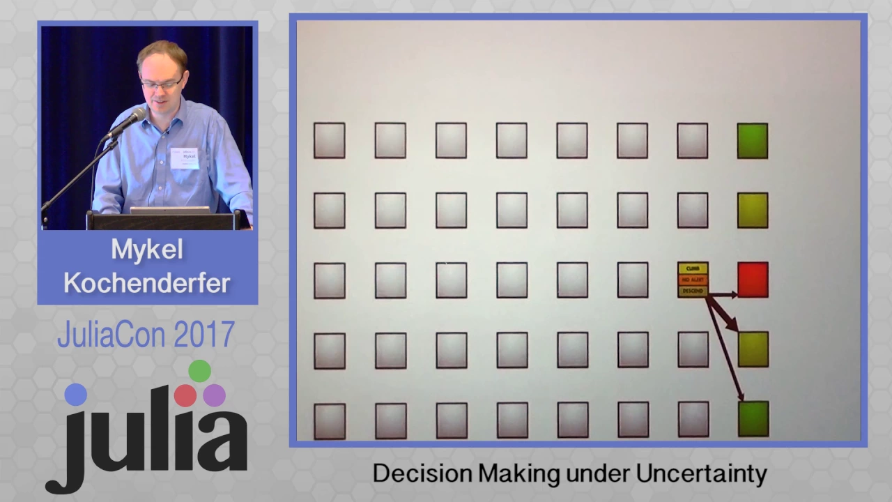
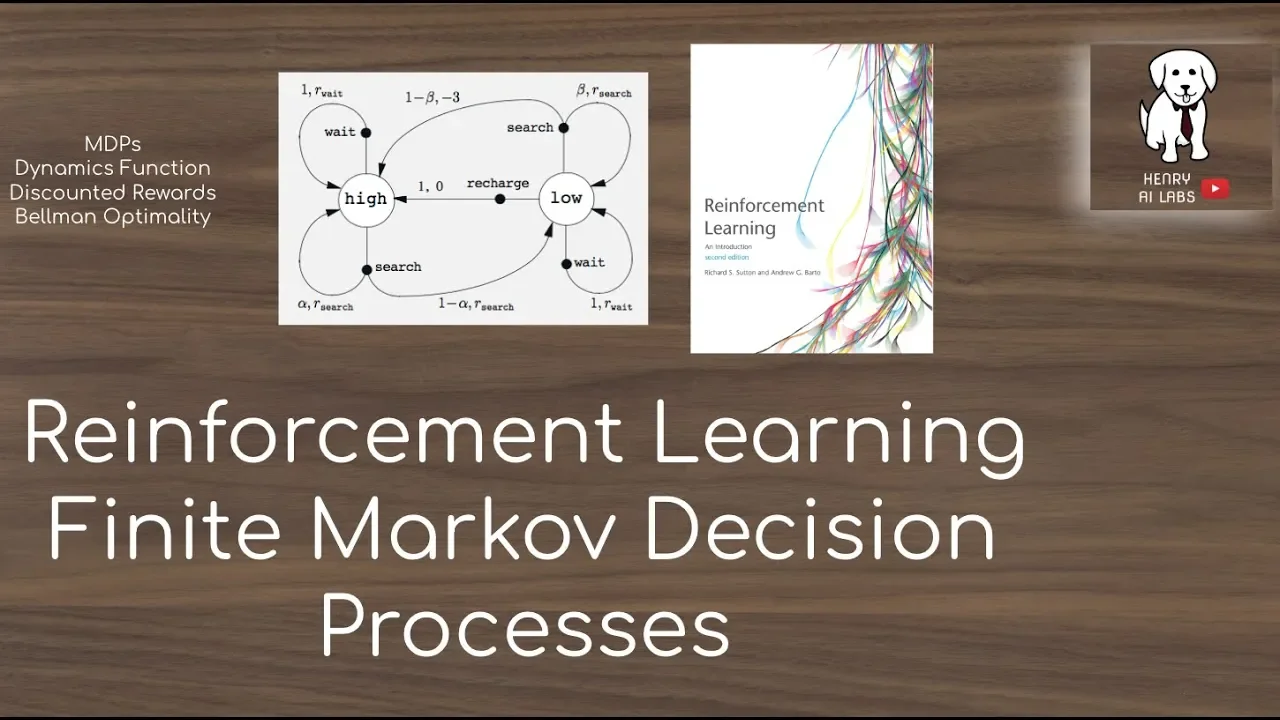
The concept of Markov Decision Processes (MDPs) as the mathematical framework for decision-making under uncertainty.
Fundamental probability concepts, particularly expected values and discounting future rewards (discount factor gamma).
Basic data structures, specifically 2D arrays or matrices, to understand how a Q-table stores and updates values.
Exploration vs. Exploitation strategies, such as the Epsilon-Greedy algorithm, to balance search and optimization.
Deep Q-Networks (DQN), which use deep neural networks as function approximators for continuous or high-dimensional state spaces.
On-policy vs. Off-policy learning, specifically comparing Q-Learning with the SARSA algorithm.
Practical implementation of Q-learning in benchmark environments, such as OpenAI Gym's Gridworld or FrozenLake.
82.4K views2.5Klikes11:54Original Release: 2023-11-07
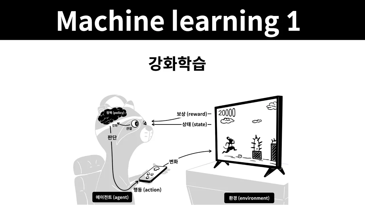
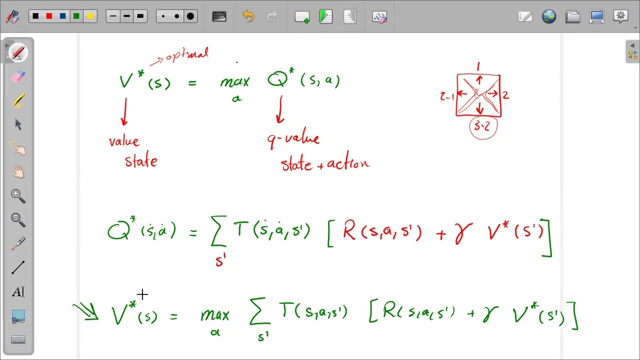
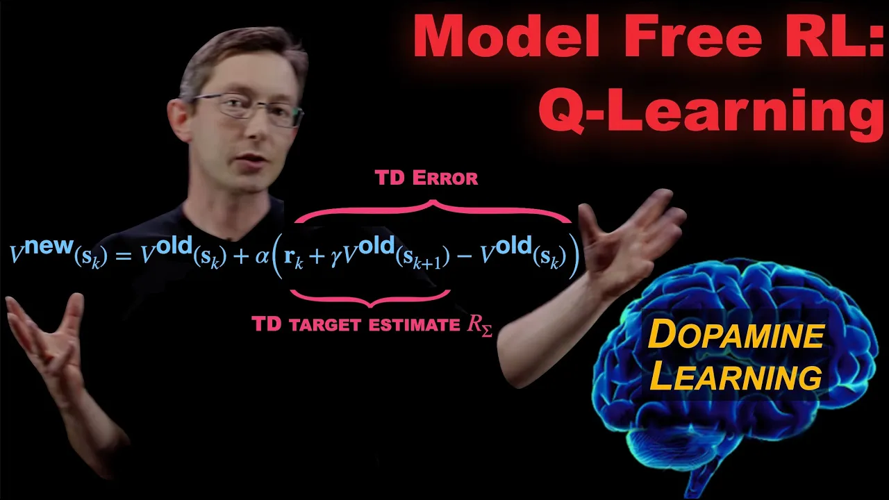
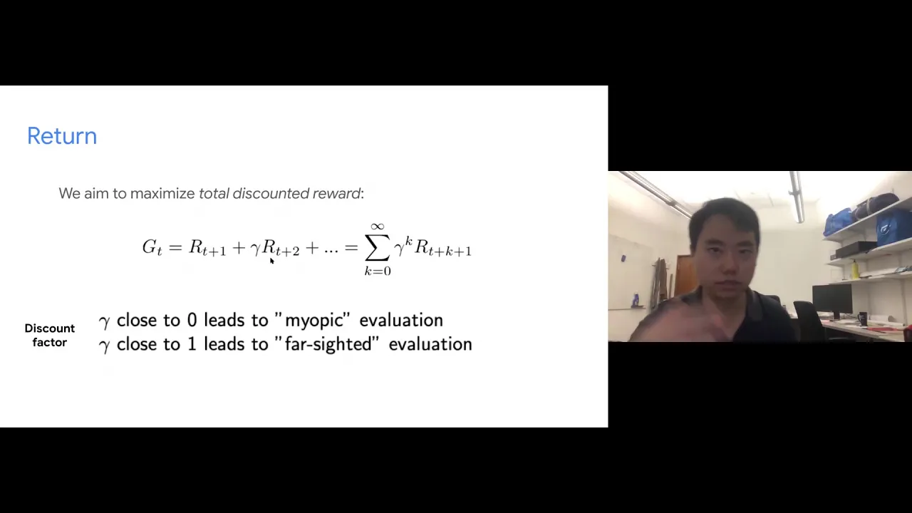
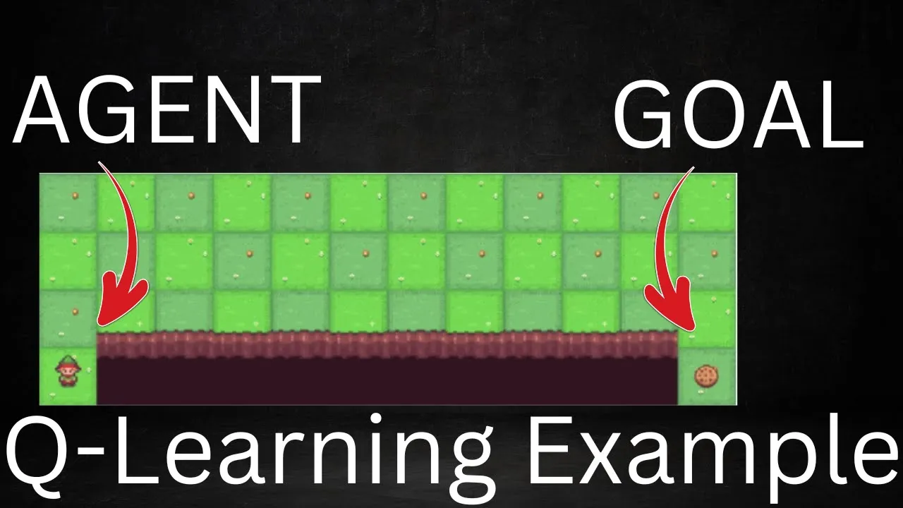
hello everyone and welcome to another episode of Code Emporium where we're going to talk about q-learning arguably one of the most popular Concepts in reinforcement learning so let's get to it now throughout the series on reinforcement learning which you can check the playlist down in the description below we have discussed that machines can learn in primarily three different ways which are known as the machine learning paradigms so the first one is supervised learning that is we have a dumb model we have data we have a label we use that to train said dumb model in order to recognize patterns between the data and the label and this is primarily used in classification and regression type problems the second is unsupervised learning where we have data but we don't have a label and the primary objective is to understand patterns within the data so this is used in clustering and dimensionality reduction among others and then the third pillar is reinforcement learning from the text B reinforcement learning is learning what to do that is how to map situations to actions so as to maximize a numerical reward signal now we can break reinforcement learning algorithms down into two types that is the value based methods and the policy based methods remember at the end of the day we're trying to maximize total reward so value based methods will determine a value function that quantifies this total reward and using this value function it'll determine the optimal policy policy based methods will determine an optimal policy directly and optimal policy is the policy that maximizes the total reward and just to note that policy is how an agent behaves in a given situation or state now Q learning is a value-based reinforcement learning method to solve problems and so we can dive a little bit more into these value based methods so value based methods determine a value function that that in turn determines a policy that's going to maximize Total Rewards a value function is a function so it has some inputs and it generates an output and depending on the inputs there are two types of value functions we have state value functions represented by V and then we have state action functions represented by q but now States actions what are those a state is a snapshot of the environment and an action is the decision taken by an agent in an environment so the state value function will take a state as input and output a real number whereas the state action value function will take the state and action as input and it'll output a real number so this real number is also known as a q value ooh Q so we're getting close to Q learning here now the state value that is VFS will quantify how good is it to be in a given State s whereas the state action value or Q value will quantify how good is it to be in a state s and then take an action a in this state for Q learning we are interested in learning the state action value function because it's a function you can think of it more easily as a table of rows being States and columns being possible actions and each cell value will actually be the Q Val value for that given State and action and the goal of Q learning is to effectively learn these Q values such that the total reward is maximized so let's see how it works with this grid world so this here is a fully observable environment with nine squares and there's A+ 10 reward square a minus 10 poison square and other rewards is -1 for any other Square now the goal of our agent is to to get to this + 10 reward spot in the best possible way and more technically we want the agent to learn an optimal policy this is known as the target policy and let's say that in order to learn this optimal policy we want to use Q learning to do this and so we need to make use of this Q table let's initialize these values to arbitrary values now note that these values could also be loaded by some other agent that explored the environment previously but for now let's just keep them arbitrary now let's say that the agent starts in the first cell at State S1 and it takes an action based on an exploration policy this means that the actions that an agent takes is simply based on random chance and the agent won't just choose a state because it has a high Q value for example and this policy is known as the behavior policy and it can be just about anything if the agent is in a state S1 it can take an action of either going right or going down and because the policy is random let's say that the agent made the decision to go right so the action is taken and then when taking the action the agent transitions into another state and let's say that this another state is S2 and on doing so it also receives a reward of1 now let's calculate the observed Q value so this is given by the Bellman equation now the Bellman equation defines a recursive relationship between Q values and for more information you can check out my video on the topic but for now the Q value for this state S1 and right is given by the sum of the reward of State S2 Plus the maximum Future q value for that state S2 that we can get and GMA here is a discount Factor just to show how much we want to Value the current reward over future rewards and so if we just plug in some values so the reward from S2 is -1 let's say that gamma that discount factor is 0.1 and then we multiply that by the maximum possible Q value that we can get from State S2 now looking at our Q table we can see that we get the maximum Q value by going down from the state S2 which is 1.5 so substituting 1.5 in our equation we'll get the overall Q value as 0.85 this is the observe value for q1 State S1 and going right but the value at the table for this specific Q value is one there's clearly a difference and this difference is an error that is known as a temporal difference error it's called called the temporal difference error because we are comparing Q values of two different time steps and their difference is the error hence the name for more information on this topic I created another video right here but for now temporal difference eror is now going to be the observed value minus the expected value which will turn out to be - 1.85 We Now update the Q value in the table based on the formula that looks like a gradient update Rule and here Alpha is going to be the step size or the learning rate so to speak and it defines how much in every time step are we willing to change these Q values higher the value faster learning because bigger the updates so in this case let's also just take it to be some 0.1 and plugging in these values we get 1 which is the expected Value Plus 0.1 * the error which is 1.85 and then doing the math you will get 0.815 as the final result and so we update this single Q value in the table from 1 to 0.85 and this is the end of our first time step let's now walk through another time step just to make sure that we understand what's going on so let's say that now we're in a state S2 in time step two and we can take the action of either going right left or down and the policy We are following is now random so let's say that we choose to go down we take the action and then on taking the action the agent will transition into another state let's say it's S6 and it receives a reward of -1 now let's calculate the observed Q value that is given by the Bellman equation so the Q value observed is going to be the reward in transitioning into State S6 plus the discounted maximum value that we can obtain for State X6 and so we know that the reward for State S6 is -1 and from our table when we are in state S6 the maximum possible Q value is going to be 1.7 and this is the value if we choose to go in the downward direction from S6 so we substitute that in the equation and we get 0.83 now this is the observed value but the expected value that is stored in the table for this cell is 1.5 and so the temporal difference there is going to be the difference of The observed minus the expected 0.83 minus 1.5 and we'll get - 2.33 and now we are going to now plug this value into our update rule for the temporal difference error and so this gives us a 1.5 for the current Q value expected plus 0.1 times the temporal difference Arrow of - 2.33 doing the math you get 1.26 7 and so we update the single Q value in our table and this is the end of our second time step we repeat this until the sequence of steps is over that is until we get to the plus 10 spot or the negative - 10 spot and this sequence of steps until now is known as one episode we can then perform multiple episodes over and over again choosing random actions and effectively just learning the values of the Q table until they become more stable and effectively these Q values are learned and once they are learned an agent can take an action based on which will give us the highest Q value result and so the Q value will dictate the policy to get our reward and this new policy remember was the target policy that we were trying to achieve and note that this is different from the behavior policy that we use to explore the environment in order to learn effectively the target policy later on because we can decouple this Behavior policy for collecting data from the target policy which is used when we have an optimal Q table Q learning is known as a type of off policy Al them and so I hope CU learning makes sense at least at this surface level that's all I have for today thank you all so much for watching and if you like the video and you think I deserve it please give this video a like And subscribe for more amazing content we're at 100,000 subscribers would love to get to 150,000 subscribers real soon but thank you all so much and I will see you in another one bye-bye
Up Next
67:10
Markov Decision Processes (MDPs) Explained | CS188 Lecture 8
@CS188Spring2013
125.7K views•2013-02-15

57:48
Secure Multiparty Computation (MPC): Foundations & Challenges
@SimonsInstitute
7.3K views•2015-05-28

13:26
Proximal Policy Optimization: RL Algorithm Explained | PPO Tutorial
@CodeEmporium
41.2K views•2023-12-04

18:41
Neural Networks Explained: Math, Layers, and Learning Fundamentals
@3blue1brown
21.9M views•2017-10-05
Related Study Plans & Knowledge Roadmaps
Structured learning paths in Artificial Intelligence
artificial-intelligence
Aligning LLMs: DPO, TRL & Custom Datasets
01Foundations of Python & Machine Learning
02Transformers and Large Language Models (LLMs)
03Aligning LLMs: SFT and RLHF
+ 3 more learning modules
24h6 modules
Explore Roadmap
artificial-intelligence
Federated Learning: PyTorch, Flower & Privacy
01Python & Machine Learning Foundations
02Deep Learning Basics with PyTorch
03Introduction to Federated Learning
+ 2 more learning modules
35h5 modules
Explore Roadmap
artificial-intelligence
Securing LLMs: Guardrails AI & NeMo Gateway
01Introduction to LLMs, Python, and APIs
02Understanding LLM Vulnerabilities & Threats
03Defending LLMs with Guardrails AI
+ 2 more learning modules
15h5 modules
Explore Roadmap
artificial-intelligence
Building Recommenders: Two-Tower & Vector DBs
01Foundations of Python & Machine Learning Basics
02Introduction to Recommender Systems
03Deep Learning & Representation Learning
+ 3 more learning modules
75h6 modules
Explore Roadmap