




![[인공지능 25강] 손실함수 (크로스 엔트로피)](https://i.ytimg.com/vi/hceue0LPAN0/sddefault.jpg)


![HIMTI Responsi 2026/2027 | Machine Learning [B28] | UTS Semester Genap](https://i.ytimg.com/vi/3tgRb2nPJJw/maxresdefault.jpg)
![Normalization 모두 이해하기 [Batch Norm, Layer Norm, instance Norm]](https://i.ytimg.com/vi_webp/gyBGvqQEeNI/maxresdefault.webp)














This lecture covers advanced optimization algorithms for neural network training, including momentum (which adds velocity to gradient descent to overcome zigzagging and saddle points), RMSProp (which adapts learning rates per dimension using exponentially decaying gradient estimates), and Adam (which combines momentum with RMSProp for adaptive learning rates). The lecture also discusses regularization strategies such as dropout (randomly zeroing activations during training to prevent co-adaptation), batch normalization (normalizing intermediate activations to stabilize training), and data augmentation (applying random transformations to training data). Finally, transfer learning is introduced as a strategy to leverage pre-trained models on large datasets like ImageNet for tasks with limited data, either by fine-tuning the entire network or training only the final classification layer.
Training Neural Networks II: Optimization, Regularization & Transfer Learning
Added:- Okay, it's after 12, so I think we should get started.
Today we're going to kind of pick up where we left off last time.
Last time we talked about a lot of sort of tips and tricks involved in the nitty gritty details of training neural networks.
Today we'll pick up where we left off, and talk about a lot more of these sort of nitty gritty details about training these things.
As usual, a couple administrative notes before we get into the material.
As you all know, assignment one is already due.
Hopefully you all turned it in.
Did it go okay? Was it not okay?
Rough sentiment?
Mostly okay.
Okay, that's good.
Awesome. [laughs] We're in the process of grading those, so stay turned.
We're hoping to get grades back for those before A two is due.
Another reminder, that your project proposals are due tomorrow.
Actually, no, today at 11:59.
Make sure you send those in.
Details are on the website and on Piazza.
Also a reminder, assignment two is already out.
That'll be due a week from Thursday.
Historically, assignment two has been the longest one in the class, so if you haven't started already on assignment two, I'd recommend you take a look at that pretty soon.
Another reminder is that for assignment two, I think of a lot of you will be using Google Cloud.
Big reminder, make sure to stop your instances when you're not using them because whenever your instance is on, you get charged, and we only have so many coupons to distribute to you guys.
Anytime your instance is on, even if you're not SSH to it, even if you're not running things immediately in your Jupyter Notebook, any time that instance is on, you're going to be charged.
Just make sure that you explicitly stop your instances when you're not using them.
In this example, I've got a little screenshot of my dashboard on Google Cloud.
I need to go in there and explicitly go to the dropdown and click stop.
Just make sure that you do this when you're done working each day.
Another thing to remember is it's kind of up to you guys to keep track of your spending on Google Cloud.
In particular, instances that use GPUs are a lot more expensive than those with CPUs.
Rough order of magnitude, those GPU instances are around 90 cents to a dollar an hour.
Those are actually quite pricey.
The CPU instances are much cheaper.
The general strategy is that you probably want to make two instances, one with a GPU and one without, and then only use that GPU instance when you really need the GPU.
For example, on assignment two, most of the assignment, you should only need the CPU, so you should only use your CPU instance for that.
But then the final question, about TensorFlow or PyTorch, that will need a GPU.
This'll give you a little bit of practice with switching between multiple instances and only using that GPU when it's really necessary.
Again, just kind of watch your spending.
Try not to go too crazy on these things.
Any questions on the administrative stuff before we move on?
Question.
- [Student] How much RAM should we use?
- Question is how much RAM should we use?
I think eight or 16 gigs is probably good for everything that you need in this class.
As you scale up the number of CPUs and the number of RAM, you also end up spending more money.
If you stick with two or four CPUs and eight or 16 gigs of RAM, that should be plenty for all the homework-related stuff that you need to do.
As a quick recap, last time we talked about activation functions.
We talked about this whole zoo of different activation functions and some of their different properties.
We saw that the sigmoid, which used to be quite popular when training neural networks maybe 10 years ago or so, has this problem with vanishing gradients near the two ends of the activation function.
tanh has this similar sort of problem.
Kind of the general recommendation is that you probably want to stick with ReLU for most cases as sort of a default choice 'cause it tends to work well for a lot of different architectures.
We also talked about weight initialization.
Remember that up on the top, we have this idea that when you initialize your weights at the start of training, if those weights are initialized to be too small, then if you look at, then the activations will vanish as you go through the network because as you multiply by these small numbers over and over again, they'll all sort of decay to zero.
Then everything will be zero, learning won't happen, you'll be sad.
On the other hand, if you initialize your weights too big, then as you go through the network and multiply by your weight matrix over and over again, eventually they'll explode.
You'll be unhappy, there'll be no learning, it will be very bad.
But if you get that initialization just right, for example, using the Xavier initialization or the MSRA initialization, then you kind of keep a nice distribution of activations as you go through the network.
Remember that this kind of gets more and more important and more and more critical as your networks get deeper and deeper because as your network gets deeper, you're multiplying by those weight matrices over and over again with these more multiplicative terms.
We also talked last time about data preprocessing.
We talked about how it's pretty typical in conv nets to zero center and normalize your data so it has zero mean and unit variance.
I wanted to provide a little bit of extra intuition about why you might actually want to do this.
Imagine a simple setup where we have a binary classification problem where we want to draw a line to separate these red points from these blue points.
On the left, you have this idea where if those data points are kind of not normalized and not centered and far away from the origin, then we can still use a line to separate them, but now if that line wiggles just a little bit, then our classification is going to get totally destroyed.
That kind of means that in the example on the left, the loss function is now extremely sensitive to small perturbations in that linear classifier in our weight matrix.
We can still represent the same functions, but that might make learning quite difficult because, again, their loss is very sensitive to our parameter vector, whereas in the situation on the right, if you take that data cloud and you move it into the origin and you make it unit variance, then now, again, we can still classify that data quite well, but now as we wiggle that line a little bit, then our loss function is less sensitive to small perturbations in the parameter values.
That maybe makes optimization a little bit easier, as we'll see a little bit going forward.
By the way, this situation is not only in the linear classification case.
Inside a neural network, remember we kind of have these interleavings of these linear matrix multiplies, or convolutions, followed by non-linear activation functions.
If the input to some layer in your neural network is not centered or not zero mean, not unit variance, then again, small perturbations in the weight matrix of that layer of the network could cause large perturbations in the output of that layer, which, again, might make learning difficult.
This is kind of a little bit of extra intuition about why normalization might be important.
Because we have this intuition that normalization is so important, we talked about batch normalization, which is where we just add this additional layer inside our networks to just force all of the intermediate activations to be zero mean and unit variance.
I've sort of resummarized the batch normalization equations here with the shapes a little bit more explicitly.
Hopefully this can help you out when you're implementing this thing on assignment two.
But again, in batch normalization, we have this idea that in the forward pass, we use the statistics of the mini batch to compute a mean and a standard deviation, and then use those estimates to normalize our data on the forward pass.
Then we also reintroduce the scale and shift parameters to increase the expressivity of the layer.
You might want to refer back to this when working on assignment two.
We also talked last time a little bit about babysitting the learning process, how you should probably be looking at your loss curves during training.
Here's an example of some networks I was actually training over the weekend.
This is usually my setup when I'm working on these things.
On the left, I have some plot showing the training loss over time.
You can see it's kind of going down, which means my network is reducing the loss.
It's doing well.
On the right, there's this plot where the X axis is, again, time, or the iteration number, and the Y axis is my performance measure both on my training set and on my validation set.
You can see that as we go over time, then my training set performance goes up and up and up and up and up as my loss function goes down, but at some point, my validation set performance kind of plateaus.
This kind of suggests that maybe I'm overfitting in this situation.
Maybe I should have been trying to add additional regularization.
We also talked a bit last time about hyperparameter search.
All these networks have sort of a large zoo of hyperparameters.
It's pretty important to set them correctly.
We talked a little bit about grid search versus random search, and how random search is maybe a little bit nicer in theory because in the situation where your performance might be more sensitive, with respect to one hyperparameter than other, and random search lets you cover that space a little bit better.
We also talked about the idea of coarse to fine search, where when you're doing this hyperparameter optimization, probably you want to start with very wide ranges for your hyperparameters, only train for a couple iterations, and then based on those results, you kind of narrow in on the range of hyperparameters that are good.
Now, again, redo your search in a smaller range for more iterations.
You can kind of iterate this process to kind of hone in on the right region for hyperparameters.
But again, it's really important to, at the start, have a very coarse range to start with, where you want very, very wide ranges for all your hyperparameters.
Ideally, those ranges should be so wide that your network is kind of blowing up at either end of the range so that you know that you've searched a wide enough range for those things.
Question?
- [Student] How many [speaks too low to hear] optimize at once?
[speaks too low to hear] - The question is how many hyperparameters do we typically search at a time?
Here is two, but there's a lot more than two in these typical things.
It kind of depends on the exact model and the exact architecture, but because the number of possibilities is exponential in the number of hyperparameters, you can't really test too many at a time.
It also kind of depends on how many machines you have available.
It kind of varies from person to person and from experiment to experiment.
But generally, I try not to do this over more than maybe two or three or four at a time at most because, again, this exponential search just gets out of control.
Typically, learning rate is the really important one that you need to nail first.
Then other things, like regularization, like learning rate decay, model size, these other types of things tend to be a little bit less sensitive than learning rate.
Sometimes you might do kind of a block coordinate descent, where you go and find the good learning rate, then you go back and try to look at different model sizes.
This can help you cut down on the exponential search a little bit, but it's a little bit problem dependent on exactly which ones you should be searching over in which order.
More questions?
- [Student] [speaks too low to hear] Another parameter, but then changing that other parameter, two or three other parameters, makes it so that your learning rate or the ideal learning rate is still [speaks too low to hear].
- Question is how often does it happen where when you change one hyperparameter, then the other, the optimal values of the other hyperparameters change?
That does happen sometimes, although for learning rates, that's typically less of a problem.
For learning rates, typically you want to get in a good range, and then set it maybe even a little bit lower than optimal, and let it go for a long time.
Then if you do that, combined with some of the fancier optimization strategies that we'll talk about today, then a lot of models tend to be a little bit less sensitive to learning rate once you get them in a good range.
Sorry, did you have a question in front, as well?
- [Student] [speaks too low to hear] - The question is what's wrong with having a small learning rate and increasing the number of epochs?
The answer is that it might take a very long time. [laughs] - [Student] [speaks too low to hear] - Intuitively, if you set the learning rate very low and let it go for a very long time, then this should, in theory, always work.
But in practice, those factors of 10 or 100 actually matter a lot when you're training these things.
Maybe if you got the right learning rate, you could train it in six hours, 12 hours or a day, but then if you just were super safe and dropped it by a factor of 10 or by a factor of 100, now that one-day training becomes 100 days of training.
That's three months.
That's not going to be good.
When you're taking these intro computer science classes, they always kind of sweep the constants under the rug, but when you're actually thinking about training things, those constants end up mattering a lot.
Another question?
- [Student] If you have a low learning rate, [speaks too low to hear].
- Question is for a low learning rate, are you more likely to be stuck in local optima?
I think that makes some intuitive sense, but in practice, that seems not to be much of a problem.
I think we'll talk a bit more about that later today.
Today I wanted to talk about a couple other really interesting and important topics when we're training neural networks.
In particular, I wanted to talk, we've kind of alluded to this fact of fancier, more powerful optimization algorithms a couple times.
I wanted to spend some time today and really dig into those and talk about what are the actual optimization algorithms that most people are using these days.
We also touched on regularization in earlier lectures.
This concept of making your network do additional things to reduce the gap between train and test error.
I wanted to talk about some more strategies that people are using in practice of regularization, with respect to neural networks.
Finally, I also wanted to talk a bit about transfer learning, where you can sometimes get away with using less data than you think by transferring from one problem to another.
If you recall from a few lectures ago, the kind of core strategy in training neural networks is an optimization problem where we write down some loss function, which defines, for each value of the network weights, the loss function tells us how good or bad is that value of the weights doing on our problem.
Then we imagine that this loss function gives us some nice landscape over the weights, where on the right, I've shown this maybe small, two-dimensional problem, where the X and Y axes are two values of the weights.
Then the color of the plot kind of represents the value of the loss.
In this kind of cartoon picture of a two-dimensional problem, we're only optimizing over these two values, W one, W two.
The goal is to find the most red region in this case, which corresponds to the setting of the weights with the lowest loss.
Remember, we've been working so far with this extremely simple optimization algorithm, stochastic gradient descent, where it's super simple, it's three lines.
While true, we first evaluate the loss in the gradient on some mini batch of data.
Then we step, updating our parameter vector in the negative direction of the gradient because this gives, again, the direction of greatest decrease of the loss function.
Then we repeat this over and over again, and hopefully we converge to the red region and we get great errors and we're very happy.
But unfortunately, this relatively simple optimization algorithm has quite a lot of problems that actually could come up in practice.
One problem with stochastic gradient descent, imagine what happens if our objective function looks something like this, where, again, we're plotting two values, W one and W two.
As we change one of those values, the loss function changes very slowly.
As we change the horizontal value, then our loss changes slowly.
As we go up and down in this landscape, now our loss is very sensitive to changes in the vertical direction.
By the way, this is referred to as the loss having a bad condition number at this point, which is the ratio between the largest and smallest singular values of the Hessian matrix at that point.
But the intuitive idea is that the loss landscape kind of looks like a taco shell.
It's sort of very sensitive in one direction, not sensitive in the other direction.
The question is what might SGD, stochastic gradient descent, do on a function that looks like this?
If you run stochastic gradient descent on this type of function, you might get this characteristic zigzagging behavior, where because for this type of objective function, the direction of the gradient does not align with the direction towards the minima.
When you compute the gradient and take a step, you might step sort of over this line and sort of zigzag back and forth.
In effect, you get very slow progress along the horizontal dimension, which is the less sensitive dimension, and you get this zigzagging, nasty, nasty zigzagging behavior across the fast-changing dimension.
This is undesirable behavior.
By the way, this problem actually becomes much more common in high dimensions.
In this kind of cartoon picture, we're only showing a two-dimensional optimization landscape, but in practice, our neural networks might have millions, tens of millions, hundreds of millions of parameters.
That's hundreds of millions of directions along which this thing can move.
Now among those hundreds of millions of different directions to move, if the ratio between the largest one and the smallest one is bad, then SGD will not perform so nicely.
You can imagine that if we have 100 million parameters, probably the maximum ratio between those two will be quite large.
I think this is actually quite a big problem in practice for many high-dimensional problems.
Another problem with SGD has to do with this idea of local minima or saddle points.
Here I've sort of swapped the graph a little bit.
Now the X axis is showing the value of one parameter, and then the Y axis is showing the value of the loss.
In this top example, we have kind of this curvy objective function, where there's a valley in the middle.
What happens to SGD in this situation?
- [Student] [speaks too low to hear] - In this situation, SGD will get stuck because at this local minima, the gradient is zero because it's locally flat.
Now remember with SGD, we compute the gradient and step in the direction of opposite gradient, so if at our current point, the opposite gradient is zero, then we're not going to make any progress, and we'll get stuck at this point.
There's another problem with this idea of saddle points.
Rather than being a local minima, you can imagine a point where in one direction we go up, and in the other direction we go down.
Then at our current point, the gradient is zero.
Again, in this situation, the function will get stuck at the saddle point because the gradient is zero.
Although one thing I'd like to point out is that in one dimension, in a one-dimensional problem like this, local minima seem like a big problem and saddle points seem like kind of not something to worry about, but in fact, it's the opposite once you move to very high-dimensional problems because, again, if you think about you're in this 100 million dimensional space, what does a saddle point mean?
That means that at my current point, some directions the loss goes up, and some directions the loss goes down.
If you have 100 million dimensions, that's probably going to happen more frequently than, that's probably going to happen almost everywhere, basically.
Whereas a local minima says that of all those 100 million directions that I can move, every one of them causes the loss to go up.
In fact, that seems pretty rare when you're thinking about, again, these very high-dimensional problems.
Really, the idea that has come to light in the last few years is that when you're training these very large neural networks, the problem is more about saddle points and less about local minima.
By the way, this also is a problem not just exactly at the saddle point, but also near the saddle point.
If you look at the example on the bottom, you see that in the regions around the saddle point, the gradient isn't zero, but the slope is very small.
That means that if we're, again, just stepping in the direction of the gradient, and that gradient is very small, we're going to make very, very slow progress whenever our current parameter value is near a saddle point in the objective landscape.
This is actually a big problem.
Another problem with SGD comes from the S.
Remember that SGD is stochastic gradient descent.
Recall that our loss function is typically defined by computing the loss over many, many different examples.
In this case, if N is your whole training set, then that could be something like a million.
Each time computing the loss would be very, very expensive.
In practice, remember that we often estimate the loss and estimate the gradient using a small mini batch of examples.
What this means is that we're not actually getting the true information about the gradient at every time step.
Instead, we're just getting some noisy estimate of the gradient at our current point.
Here on the right, I've kind of faked this plot a little bit.
I've just added random uniform noise to the gradient at every point, and then run SGD with these noisy, messed up gradients.
This is maybe not exactly what happens with the SGD process, but it still give you the sense that if there's noise in your gradient estimates, then vanilla SGD kind of meanders around the space and might actually take a long time to get towards the minima.
Now that we've talked about a lot of these problems.
Sorry, was there a question?
- [Student] [speaks too low to hear] - The question is do all of these just go away if we use normal gradient descent?
Let's see.
I think that the taco shell problem of high condition numbers is still a problem with full batch gradient descent.
The noise.
As we'll see, we might sometimes introduce additional noise into the network, not only due to sampling mini batches, but also due to explicit stochasticity in the network, so we'll see that later.
That can still be a problem.
Saddle points, that's still a problem for full batch gradient descent because there can still be saddle points in the full objective landscape.
Basically, even if we go to full batch gradient descent, it doesn't really solve these problems.
We kind of need to think about a slightly fancier optimization algorithm that can try to address these concerns.
Thankfully, there's a really, really simple strategy that works pretty well at addressing many of these problems.
That's this idea of adding a momentum term to our stochastic gradient descent.
Here on the left, we have our classic old friend, SGD, where we just always step in the direction of the gradient.
But now on the right, we have this minor, minor variance called SGD plus momentum, which is now two equations and five lines of code, so it's twice as complicated.
But it's very simple.
The idea is that we maintain a velocity over time, and we add our gradient estimates to the velocity.
Then we step in the direction of the velocity, rather than stepping in the direction of the gradient.
This is very, very simple.
We also have this hyperparameter rho now which corresponds to friction.
Now at every time step, we take our current velocity, we decay the current velocity by the friction constant, rho, which is often something high, like.9 is a common choice.
We take our current velocity, we decay it by friction and we add in our gradient.
Now we step in the direction of our velocity vector, rather than the direction of our raw gradient vector.
This super, super simple strategy actually helps for all of these problems that we just talked about.
If you think about what happens at local minima or saddle points, then if we're imagining velocity in this system, then you kind of have this physical interpretation of this ball kind of rolling down the hill, picking up speed as it comes down.
Now once we have velocity, then even when we pass that point of local minima, the point will still have velocity, even if it doesn't have gradient.
Then we can hopefully get over this local minima and continue downward.
There's this similar intuition near saddle points, where even though the gradient around the saddle point is very small, we have this velocity vector that we've built up as we roll downhill.
That can hopefully carry us through the saddle point and let us continue rolling all the way down.
If you think about what happens in poor conditioning, now if we were to have these kind of zigzagging approximations to the gradient, then those zigzags will hopefully cancel each other out pretty fast once we're using momentum.
This will effectively reduce the amount by which we step in the sensitive direction, whereas in the horizontal direction, our velocity will just keep building up, and will actually accelerate our descent across that less sensitive dimension.
Adding momentum here can actually help us with this high condition number problem, as well.
Finally, on the right, we've repeated the same visualization of gradient descent with noise.
Here, the black is this vanilla SGD, which is sort of zigzagging all over the place, where the blue line is showing now SGD with momentum.
You can see that because we're adding it, we're building up this velocity over time, the noise kind of gets averaged out in our gradient estimates.
Now SGD ends up taking a much smoother path towards the minima, compared with the SGD, which is kind of meandering due to noise.
Question?
- [Student] [speaks too low to hear] - The question is how does SGD momentum help with the poorly conditioned coordinate?
The idea is that if you go back and look at this velocity estimate and look at the velocity computation, we're adding in the gradient at every time step.
It kind of depends on your setting of rho, that hyperparameter, but you can imagine that if the gradient is relatively small, and if rho is well behaved in this situation, then our velocity could actually monotonically increase up to a point where the velocity could now be larger than the actual gradient.
Then we might actually make faster progress along the poorly conditioned dimension.
Kind of one picture that you can have in mind when we're doing SGD plus momentum is that the red here is our current point.
At our current point, we have some red vector, which is the direction of the gradient, or rather our estimate of the gradient at the current point.
Green is now the direction of our velocity vector.
Now when we do the momentum update, we're actually stepping according to a weighted average of these two.
This helps overcome some noise in our gradient estimate.
There's a slight variation of momentum that you sometimes see, called Nesterov accelerated gradient, also sometimes called Nesterov momentum.
That switches up this order of things a little bit.
In sort of normal SGD momentum, we imagine that we estimate the gradient at our current point, and then take a mix of our velocity and our gradient.
With Nesterov accelerated gradient, you do something a little bit different.
Here, you start at the red point.
You step in the direction of where the velocity would take you.
You evaluate the gradient at that point.
Then you go back to your original point and kind of mix together those two.
This is kind of a funny interpretation, but you can imagine that you're kind of mixing together information a little bit more.
If your velocity direction was actually a little bit wrong, it lets you incorporate gradient information from a little bit larger parts of the objective landscape.
This also has some really nice theoretical properties when it comes to convex optimization, but those guarantees go a little bit out the window once it comes to non-convex problems like neural networks.
Writing it down in equations, Nesterov momentum looks something like this, where now to update our velocity, we take a step, according to our previous velocity, and evaluate that gradient there.
Now when we take our next step, we actually step in the direction of our velocity that's incorporating information from these multiple points.
Question?
- [Student] [speaks too low to hear] - Oh, sorry.
The question is what's a good initialization for the velocity?
This is almost always zero.
It's not even a hyperparameter.
Just set it to zero and don't worry.
Another question?
- [Student] [speaks too low to hear] - Intuitively, the velocity is kind of a weighted sum of your gradients that you've seen over time.
- [Student] [speaks too low to hear] - With more recent gradients being weighted heavier.
At every time step, we take our old velocity, we decay by friction and we add in our current gradient.
You can kind of think of this as a smooth moving average of your recent gradients with kind of a exponentially decaying weight on your gradients going back in time.
This Nesterov formulation is a little bit annoying 'cause if you look at this, normally when you have your loss function, you want to evaluate your loss and your gradient at the same point.
Nesterov breaks this a little bit.
It's a little bit annoying to work with.
Thankfully, there's a cute change of variables you can do.
If you do the change of variables and reshuffle a little bit, then you can write Nesterov momentum in a slightly different way that now, again, lets you evaluate the loss and the gradient at the same point always.
Once you make this change of variables, you get kind of a nice interpretation of Nesterov, which is that here in the first step, this looks exactly like updating the velocity in the vanilla SGD momentum case, where we have our current velocity, we evaluate gradient at the current point and mix these two together in a decaying way.
Now in the second update, now when we're actually updating our parameter vector, if you look at the second equation, we have our current point plus our current velocity plus a weighted difference between our current velocity and our previous velocity.
Here, Nesterov momentum is kind of incorporating some kind of error-correcting term between your current velocity and your previous velocity.
If we look at SGD, SGD momentum and Nesterov momentum on this kind of simple problem, compared with SGD, we notice that SGD kind of takes this, SGD is in the black, kind of taking this slow progress toward the minima.
The blue and the green show momentum and Nesterov.
These have this behavior of kind of overshooting the minimum 'cause they're building up velocity going past the minimum, and then kind of correcting themselves and coming back towards the minima.
Question?
- [Student] [speaks too low to hear] - The question is this picture looks good, but what happens if your minima call lies in this very narrow basin?
Will the velocity just cause you to skip right over that minima?
That's actually a really interesting point, and the subject of some recent theoretical work, but the idea is that maybe those really sharp minima are actually bad minima.
We don't want to even land in those 'cause the idea is that maybe if you have a very sharp minima, that actually could be a minima that overfits more.
If you imagine that we doubled our training set, the whole optimization landscape would change, and maybe that very sensitive minima would actually disappear if we were to collect more training data.
We kind of have this intuition that we maybe want to land in very flat minima because those very flat minima are probably more robust as we change the training data.
Those flat minima might actually generalize better to testing data.
This is again, sort of very recent theoretical work, but that's actually a really good point that you bring it up.
In some sense, it's actually a feature and not a bug that SGD momentum actually skips over those very sharp minima.
That's actually a good thing, believe it or not.
Another thing you can see is if you look at the difference between momentum and Nesterov here, you can see that because of the correction factor in Nesterov, maybe it's not overshooting quite as drastically, compared to vanilla momentum.
There's another kind of common optimization strategy is this algorithm called AdaGrad, which John Duchi, who's now a professor here, worked on during his Ph.D.
The idea with AdaGrad is that as you, during the course of the optimization, you're going to keep a running estimate or a running sum of all the squared gradients that you see during training.
Now rather than having a velocity term, instead we have this grad squared term.
During training, we're going to just keep adding the squared gradients to this grad squared term.
Now when we update our parameter vector, we'll divide by this grad squared term when we're making our update step.
The question is what does this kind of scaling do in this situation where we have a very high condition number?
- [Student] [speaks too low to hear] - The idea is that if we have two coordinates, one that always has a very high gradient and one that always has a very small gradient, then as we add the sum of the squares of the small gradient, we're going to be dividing by a small number, so we'll accelerate movement along the slow dimension, along the one dimension.
Then along the other dimension, where the gradients tend to be very large, then we'll be dividing by a large number, so we'll kind of slow down our progress along the wiggling dimension.
But there's kind of a problem here.
That's the question of what happens with AdaGrad over the course of training, as t gets larger and larger and larger?
- [Student] [speaks too low to hear] - With AdaGrad, the steps actually get smaller and smaller and smaller because we just continue updating this estimate of the squared gradients over time, so this estimate just grows and grows and grows monotonically over the course of training.
Now this causes our step size to get smaller and smaller and smaller over time.
Again, in the convex case, there's some really nice theory showing that this is actually really good 'cause in the convex case, as you approach a minimum, you kind of want to slow down so you actually converge.
That's actually kind of a feature in the convex case.
But in the non-convex case, that's a little bit problematic because as you come towards a saddle point, you might get stuck with AdaGrad, and then you kind of no longer make any progress.
There's a slight variation of AdaGrad, called RMSProp, that actually addresses this concern a little bit.
Now with RMSProp, we still keep this estimate of the squared gradients, but instead of just letting that squared estimate continually accumulate over training, instead, we let that squared estimate actually decay.
This ends up looking kind of like a momentum update, except we're having kind of momentum over the squared gradients, rather than momentum over the actual gradients.
Now with RMSProp, after we compute our gradient, we take our current estimate of the grad squared, we multiply it by this decay rate, which is commonly something like.9 or.99.
Then we add in this one minus the decay rate of our current squared gradient.
Now over time, you can imagine that.
Then again, when we make our step, the step looks exactly the same as AdaGrad, where we divide by the squared gradient in the step to again have this nice property of accelerating movement along the one dimension, and slowing down movement along the other dimension.
But now with RMSProp, because these estimates are leaky, then it kind of addresses the problem of maybe always slowing down where you might not want to.
Here again, we're kind of showing our favorite toy problem with SGD in black, SGD momentum in blue and RMSProp in red.
You can see that RMSProp and SGD momentum are both doing much better than SGD, but their qualitative behavior is a little bit different.
With SGD momentum, it kind of overshoots the minimum and comes back, whereas with RMSProp, it's kind of adjusting its trajectory such that we're making approximately equal progress among all the dimensions.
By the way, you can't actually tell, but this plot is also showing AdaGrad in green with the same learning rate, but it just gets stuck due to this problem of continually decaying learning rates.
In practice, AdaGrad is maybe not so common for many of these things.
That's a little bit of an unfair comparison of AdaGrad.
Probably you need to increase the learning rate with AdaGrad, and then it would end up looking kind of like RMSProp in this case.
But in general, we tend not to use AdaGrad so much when training neural networks.
Question?
- [Student] [speaks too low to hear] - The answer is yes, this problem is convex, but in this case, it's a little bit of an unfair comparison because the learning rates are not so comparable among the methods.
I've been a little bit unfair to AdaGrad in this visualization by showing the same learning rate between the different algorithms, when probably you should have separately turned the learning rates per algorithm.
We saw in momentum, we had this idea of velocity, where we're building up velocity by adding in the gradients, and then stepping in the direction of the velocity.
We saw with AdaGrad and RMSProp that we had this other idea, of building up an estimate of the squared gradients, and then dividing by the squared gradients.
Then these both seem like good ideas on their own.
Why don't we just stick 'em together and use them both?
Maybe that would be even better.
That brings us to this algorithm called Adam, or rather brings us very close to Adam.
We'll see in a couple slides that there's a slight correction we need to make here.
Here with Adam, we maintain an estimate of the first moment and the second moment.
Now in the red, we make this estimate of the first moment as a weighed sum of our gradients.
We have this moving estimate of the second moment, like AdaGrad and like RMSProp, which is a moving estimate of our squared gradients.
Now when we make our update step, we step using both the first moment, which is kind of our velocity, and also divide by the second moment, or rather the square root of the second moment, which is this squared gradient term.
This idea of Adam ends up looking a little bit like RMSProp plus momentum, or ends up looking like momentum plus second squared gradients.
It kind of incorporates the nice properties of both.
But there's a little bit of a problem here.
That's the question of what happens at the very first time step?
At the very first time step, you can see that at the beginning, we've initialized our second moment with zero.
Now after one update of the second moment, typically this beta two, second moment decay rate, is something like.9 or.99, something very close to one.
After one update, our second moment is still very, very close to zero.
Now when we're making our update step here and we divide by our second moment, now we're dividing by a very small number.
We're making a very, very large step at the beginning.
This very, very large step at the beginning is not really due to the geometry of the problem.
It's kind of an artifact of the fact that we initialized our second moment estimate was zero.
Question?
- [Student] [speaks too low to hear] - That's true.
The comment is that if your first moment is also very small, then you're multiplying by small and you're dividing by square root of small squared, so what's going to happen?
They might cancel each other out, you might be okay.
That's true.
Sometimes these cancel each other out and you're okay, but sometimes this ends up in taking very large steps right at the beginning.
That can be quite bad.
Maybe you initialize a little bit poorly.
You take a very large step.
Now your initialization is completely messed up, and then you're in a very bad part of the objective landscape and you just can't converge from there.
Question?
- [Student] [speaks too low to hear] - The idea is what is this 10 to the minus seven term in the last equation?
That's actually appeared in AdaGrad, RMSProp and Adam.
The idea is that we're dividing by something.
We want to make sure we're not dividing by zero, so we always add a small positive constant to the denominator, just to make sure we're not dividing by zero.
That's technically a hyperparameter, but it tends not to matter too much, so just setting 10 to minus seven, 10 to minus eight, something like that, tends to work well.
With Adam, remember we just talked about this idea of at the first couple steps, it gets very large, and we might take very large steps and mess ourselves up.
Adam also adds this bias correction term to avoid this problem of taking very large steps at the beginning.
You can see that after we update our first and second moments, we create an unbiased estimate of those first and second moments by incorporating the current time step, t.
Now we actually make our step using these unbiased estimates, rather than the original first and second moment estimates.
This gives us our full form of Adam.
By the way, Adam is a really, [laughs] really good optimization algorithm, and it works really well for a lot of different problems, so that's kind of my default optimization algorithm for just about any new problem that I'm tackling.
In particular, if you set beta one equals.9, beta two equals.999, learning rate one e minus three or five e minus four, that's a great staring point for just about all the architectures I've ever worked with.
Try that.
That's a really good place to start, in general.
[laughs] If we actually plot these things out and look at SGD, SGD momentum, RMSProp and Adam on the same problem, you can see that Adam, in the purple here, kind of combines elements of both SGD momentum and RMSProp.
Adam kind of overshoots the minimum a little bit like SGD momentum, but it doesn't overshoot quite as much as momentum.
Adam also has this similar behavior of RMSProp of kind of trying to curve to make equal progress along all dimensions.
Maybe in this small two-dimensional example, Adam converged about similarly to other ones, but you can see qualitatively that it's kind of combining the behaviors of both momentum and RMSProp.
Any questions about optimization algorithms?
- [Student] [speaks too low to hear] They still take a very long time to train.
[speaks too low to hear] - The question is what does Adam not fix?
Would these neural networks are still large, they still take a long time to train.
There can still be a problem.
In this picture where we have this landscape of things looking like ovals, if you imagine that we're kind of making estimates along each dimension independently to allow us to speed up or slow down along different coordinate axes, but one problem is that if that taco shell is kind of tilted and is not axis aligned, then we're still only making estimates along the individual axes independently.
That corresponds to taking your rotated taco shell and squishing it horizontally and vertically, but you can't actually unrotate it.
In cases where you have this kind of rotated picture of poor conditioning, then Adam or any of these other algorithms really can't address that, that concern.
Another thing that we've seen in all these optimization algorithms is learning rate as a hyperparameter.
We've seen this picture before a couple times, that as you use different learning rates, sometimes if it's too high, it might explode in the yellow.
If it's a very low learning rate, in the blue, it might take a very long time to converge.
It's kind of tricky to pick the right learning rate.
This is a little bit of a trick question because we don't actually have to stick with one learning rate throughout the course of training.
Sometimes you'll see people decay the learning rates over time, where we can kind of combine the effects of these different curves on the left, and get the nice properties of each.
Sometimes you'll start with a higher learning rate near the start of training, and then decay the learning rate and make it smaller and smaller throughout the course of training.
A couple strategies for these would be a step decay, where at 100,000th iteration, you just decay by some factor and you keep going.
You might see an exponential decay, where you continually decay during training.
You might see different variations of continually decaying the learning rate during training.
If you look at papers, especially the resonate paper, you often see plots that look kind of like this, where the loss is kind of going down, then dropping, then flattening again, then dropping again.
What's going on in these plots is that they're using a step decay learning rate, where at these parts where it plateaus and then suddenly drops again, those are the iterations where they dropped the learning rate by some factor.
This idea of dropping the learning rate, you might imagine that it got near some good region, but now the gradients got smaller, it's kind of bouncing around too much.
Then if we drop the learning rate, it lets it slow down and continue to make progress down the landscape.
This tends to help in practice sometimes.
Although one thing to point out is that learning rate decay is a little bit more common with SGD momentum, and a little bit less common with something like Adam.
Another thing I'd like to point out is that learning rate decay is kind of a second-order hyperparameter.
You typically should not optimize over this thing from the start.
Usually when you're kind of getting networks to work at the beginning, you want to pick a good learning rate with no learning rate decay from the start.
Trying to cross-validate jointly over learning rate decay and initial learning rate and other things, you'll just get confused.
What you do for setting learning rate decay is try with no decay, see what happens.
Then kind of eyeball the loss curve and see where you think you might need decay.
Another thing I wanted to mention briefly is this idea of all these algorithms that we've talked about are first-order optimization algorithms.
In this picture, in this one-dimensional picture, we have this kind of curvy objective function at our current point in red.
What we're basically doing is computing the gradient at that point.
We're using the gradient information to compute some linear approximation to our function, which is kind of a first-order Taylor approximation to our function.
Now we pretend that the first-order approximation is our actual function, and we make a step to try to minimize the approximation.
But this approximation doesn't hold for very large regions, so we can't step too far in that direction.
But really, the idea here is that we're only incorporating information about the first derivative of the function.
You can actually go a little bit fancier.
There's this idea of second-order approximation, where we take into account both first derivative and second derivative information.
Now we make a second-order Taylor approximation to our function and kind of locally approximate our function with a quadratic.
Now with a quadratic, you can step right to the minimum, and you're really happy.
That's this idea of second-order optimization.
When you generalize this to multiple dimensions, you get something called the Newton step, where you compute this Hessian matrix, which is a matrix of second derivatives, and you end up inverting this Hessian matrix in order to step directly to the minimum of this quadratic approximation to your function.
Does anyone spot something that's quite different about this update rule, compared to the other ones that we've seen?
- [Student] [speaks too low to hear] - This doesn't have a learning rate.
That's kind of cool.
We're making this quadratic approximation and we're stepping right to the minimum of the quadratic.
At least in this vanilla version of Newton's method, you don't actually need a learning rate.
You just always step to the minimum at every time step.
However, in practice, you might end up, have a learning rate anyway because, again, that quadratic approximation might not be perfect, so you might only want to step in the direction towards the minimum, rather than actually stepping to the minimum, but at least in this vanilla version, it doesn't have a learning rate.
But unfortunately, this is maybe a little bit impractical for deep learning because this Hessian matrix is N by N, where N is the number of parameters in your network.
If N is 100 million, then 100 million squared is way too big.
You definitely can't store that in memory, and you definitely can't invert it.
In practice, people sometimes use these quasi-Newton methods that, rather than working with the full Hessian and inverting the full Hessian, they work with approximations.
Low-rank approximations are common.
You'll sometimes see these for some problems.
L-BFGS is one particular second-order optimizer that has this approximate second, keeps this approximation of the Hessian that you'll sometimes see, but in practice, it doesn't work too well for many deep learning problems because these approximations, these second-order approximations, don't really handle the stochastic case very much, very nicely.
They also tend not to work so well with non-convex problems.
I don't want to get into that right now too much.
In practice, what you should really do is probably Adam is a really good choice for many different neural network things, but if you're in a situation where you can afford to do full batch updates, and you know that your problem doesn't have really any stochasticity, then L-BFGS is kind of a good choice.
L-BFGS doesn't really get used for training neural networks too much, but as we'll see in a couple of lectures, it does sometimes get used for things like style transfer, where you actually have less stochasticity and fewer parameters, but you still want to solve an optimization problem.
All of these strategies we've talked about so far are about reducing training error.
All these optimization algorithms are really about driving down your training error and minimizing your objective function, but we don't really care about training error that much.
Instead, we really care about our performance on unseen data.
We really care about reducing this gap between train and test error.
The question is once we're already good at optimizing our objective function, what can we do to try to reduce this gap and make our model perform better on unseen data?
One really quick and dirty, easy thing to try is this idea of model ensembles that sometimes works across many different areas in machine learning.
The idea is pretty simple.
Rather than having just one model, we'll train 10 different models independently from different initial random restarts.
Now at test time, we'll run our data through all of the 10 models and average the predictions of those 10 models.
Adding these multiple models together tends to reduce overfitting a little bit and tend to improve performance a little bit, typically by a couple percent.
This is generally not a drastic improvement, but it is a consistent improvement.
You'll see that in competitions, like ImageNet and other things like that, using model ensembles is very common to get maximal performance.
You can actually get a little bit creative with this.
Sometimes rather than training separate models independently, you can just keep multiple snapshots of your model during the course of training, and then use these as your ensembles.
Then you still, at test time, need to average the predictions of these multiple snapshots, but you can collect the snapshots during the course of training.
There's actually a very nice paper being presented at ICLR this week that kind of has a fancy version of this idea, where we use a crazy learning rate schedule, where our learning rate goes very slow, then very fast, then very slow, then very fast.
The idea is that with this crazy learning rate schedule, then over the course of training, the model might be able to converge to different regions in the objective landscape that all are reasonably good.
If you do an ensemble over these different snapshots, then you can improve your performance quite nicely, even though you're only training the model once.
Questions?
- [Student] [speaks too low to hear] - The question is, it's bad when there's a large gap between error 'cause that means you're overfitting, but if there's no gap, then is that also maybe bad?
Do we actually want some small, optimal gap between the two?
We don't really care about the gap.
What we really care about is maximizing the performance on the validation set.
What tends to happen is that if you don't see a gap, then you could have improved your absolute performance, in many cases, by overfitting a little bit more.
There's this weird correlation between the absolute performance on the validation set and the size of that gap.
We only care about absolute performance.
Question in the back?
- [Student] Are hyperparameters the same for the ensemble?
- Are the hyperparameters the same for the ensembles?
That's a good question.
Sometimes they're not.
You might want to try different sizes of the model, different learning rates, different regularization strategies and ensemble across these different things.
That actually does happen sometimes.
Another little trick you can do sometimes is that during training, you might actually keep an exponentially decaying average of your parameter vector itself to kind of have a smooth ensemble of your own network during training.
Then use this smoothly decaying average of your parameter vector, rather than the actual checkpoints themselves.
This is called Polyak averaging, and it sometimes helps a little bit.
It's just another one of these small tricks you can sometimes add, but it's not maybe too common in practice.
Another question you might have is that how can we actually improve the performance of single models?
When we have ensembles, we still need to run, like, 10 models at test time.
That's not so great.
We really want some strategies to improve the performance of our single models.
That's really this idea of regularization, where we add something to our model to prevent it from fitting the training data too well in the attempts to make it perform better on unseen data.
We've seen a couple ideas, a couple methods for regularization already, where we add some explicit extra term to the loss.
Where we have this one term telling the model to fit the data, and another term that's a regularization term.
You saw this in homework one, where we used L2 regularization.
As we talked about in lecture a couple lectures ago, this L2 regularization doesn't really make maybe a lot of sense in the context of neural networks.
Sometimes we use other things for neural networks.
One regularization strategy that's super, super common for neural networks is this idea of dropout.
Dropout is super simple.
Every time we do a forward pass through the network, at every layer, we're going to randomly set some neurons to zero.
Every time we do a forward pass, we'll set a different random subset of the neurons to zero.
This kind of proceeds one layer at a time.
We run through one layer, we compute the value of the layer, we randomly set some of them to zero, and then we continue up through the network.
Now if you look at this fully connected network on the left versus a dropout version of the same network on the right, you can see that after we do dropout, it kind of looks like a smaller version of the same network, where we're only using some subset of the neurons.
This subset that we use varies at each iteration, at each forward pass.
Question?
- [Student] [speaks too low to hear] - The question is what are we setting to zero?
It's the activations.
Each layer is computing previous activation times the weight matrix gives you our next activation.
Then you just take that activation, set some of them to zero, and then your next layer will be partially zeroed activations times another matrix give you your next activations.
Question?
- [Student] [speaks too low to hear] - Question is which layers do you do this on?
It's more common in fully connected layers, but you sometimes see this in convolutional layers, as well.
When you're working in convolutional layers, sometimes instead of dropping each activation randomly, instead you sometimes might drop entire feature maps randomly.
In convolutions, you have this channel dimension, and you might drop out entire channels, rather than random elements.
Dropout is kind of super simple in practice.
It only requires adding two lines, one line per dropout call.
Here we have a three-layer neural network, and we've added dropout.
You can see that all we needed to do was add this extra line where we randomly set some things to zero.
This is super easy to implement.
But the question is why is this even a good idea?
We're seriously messing with the network at training time by setting a bunch of its values to zero.
How can this possibly make sense?
One sort of slightly hand wavy idea that people have is that dropout helps prevent co-adaptation of features.
Maybe if you imagine that we're trying to classify cats, maybe in some universe, the network might learn one neuron for having an ear, one neuron for having a tail, one neuron for the input being furry.
Then it kind of combines these things together to decide whether or not it's a cat.
But now if we have dropout, then in making the final decision about catness, the network cannot depend too much on any of these one features.
Instead, it kind of needs to distribute its idea of catness across many different features.
This might help prevent overfitting somehow.
Another interpretation of dropout that's come out a little bit more recently is that it's kind of like doing model ensembling within a single model.
If you look at the picture on the left, after you apply dropout to the network, we're kind of computing this subnetwork using some subset of the neurons.
Now every different potential dropout mask leads to a different potential subnetwork.
Now dropout is kind of learning a whole ensemble of networks all at the same time that all share parameters.
By the way, because of the number of potential dropout masks grows exponentially in the number of neurons, you're never going to sample all of these things.
This is really a gigantic, gigantic ensemble of networks that are all being trained simultaneously.
Then the question is what happens at test time?
Once we move to dropout, we've kind of fundamentally changed the operation of our neural network.
Previously, we've had our neural network, f, be a function of the weights, w, and the inputs, x, and then produce the output, y.
But now, our network is also taking this additional input, z, which is some random dropout mask.
That z is random.
Having randomness at test time is maybe bad.
Imagine that you're working at Facebook, and you want to classify the images that people are uploading.
Then today, your image gets classified as a cat, and tomorrow it doesn't.
That would be really weird and really bad.
You'd probably want to eliminate this stochasticity at test time once the network is already trained.
Then we kind of want to average out this randomness.
If you write this out, you can imagine actually marginalizing out this randomness with some integral, but in practice, this integral is totally intractable.
We don't know how to evaluate this thing.
You're in bad shape.
One thing you might imagine doing is approximating this integral via sampling, where you draw multiple samples of z and then average them out at test time, but this still would introduce some randomness, which is little bit bad.
Thankfully, in the case of dropout, we can actually approximate this integral in kind of a cheap way locally.
If we consider a single neuron, the output is a, the inputs are x and y, with two weights, w one, w two.
Then at test time, our value a is just w one x plus w two y.
Now imagine that we trained to this network.
During training, we used dropout with probability 1/2 of dropping our neurons.
Now the expected value of a during training, we can kind of compute analytically for this small case.
There's four possible dropout masks, and we're going to average out the values across these four masks.
We can see that the expected value of a during training is 1/2 w one x plus w two y.
There's this disconnect between this average value of w one x plus w two y at test time, and at training time, the average value is only 1/2 as much.
One cheap thing we can do is that at test time, we don't have any stochasticity.
Instead, we just multiply this output by the dropout probability.
Now these expected values are the same.
This is kind of like a local cheap approximation to this complex integral.
This is what people really commonly do in practice with dropout.
At dropout, we have this predict function, and we just multiply our outputs of the layer by the dropout probability.
The summary of dropout is that it's really simple on the forward pass.
You're just adding two lines to your implementation to randomly zero out some nodes.
Then at the test time prediction function, you just added one little multiplication by your probability.
Dropout is super simple.
It tends to work well sometimes for regularizing neural networks.
By the way, one common trick you see sometimes is this idea of inverted dropout.
Maybe at test time, you care more about efficiency, so you want to eliminate that extra multiplication by p at test time.
Then what you can do is, at test time, you use the entire weight matrix, but now at training time, instead you divide by p because training is probably happening on a GPU.
You don't really care if you do one extra multiply at training time, but then at test time, you kind of want this thing to be as efficient as possible.
Question?
- [Student] [speaks too low to hear] Now the gradient [speaks too low to hear].
- The question is what happens to the gradient during training with dropout?
You're right.
We only end up propagating the gradients through the nodes that were not dropped.
This has the consequence that when you're training with dropout, typically training takes longer because at each step, you're only updating some subparts of the network.
When you're using dropout, it typically takes longer to train, but you might have a better generalization after it's converged.
Dropout, we kind of saw is like this one concrete instantiation.
There's a little bit more general strategy for regularization where during training we add some kind of randomness to the network to prevent it from fitting the training data too well.
To kind of mess it up and prevent it from fitting the training data perfectly.
Now at test time, we want to average out all that randomness to hopefully improve our generalization.
Dropout is probably the most common example of this type of strategy, but actually batch normalization kind of fits this idea, as well.
Remember in batch normalization, during training, one data point might appear in different mini batches with different other data points.
There's a bit of stochasticity with respect to a single data point with how exactly that point gets normalized during training.
But now at test time, we kind of average out this stochasticity by using some global estimates to normalize, rather than the per mini batch estimates.
Actually batch normalization tends to have kind of a similar regularizing effect as dropout because they both introduce some kind of stochasticity or noise at training time, but then average it out at test time.
Actually, when you train networks with batch normalization, sometimes you don't use dropout at all, and just the batch normalization adds enough of a regularizing effect to your network.
Dropout is somewhat nice because you can actually tune the regularization strength by varying that parameter p, and there's no such control in batch normalization.
Another kind of strategy that fits in this paradigm is this idea of data augmentation.
During training, in a vanilla version for training, we have our data, we have our label.
We use it to update our CNN at each time step.
But instead, what we can do is randomly transform the image in some way during training such that the label is preserved.
Now we train on these random transformations of the image rather than the original images.
Sometimes you might see random horizontal flips 'cause if you take a cat and flip it horizontally, it's still a cat.
You'll randomly sample crops of different sizes from the image because the random crop of the cat is still a cat.
Then during testing, you kind of average out this stochasticity by evaluating with some fixed set of crops, often the four corners and the middle and their flips.
What's very common is that when you read, for example, papers on ImageNet, they'll report a single crop performance of their model, which is just like the whole image, and a 10 crop performance of their model, which are these five standard crops plus their flips.
Also with data augmentation, you'll sometimes use color jittering, where you might randomly vary the contrast or brightness of your image during training.
You can get a little bit more complex with color jittering, as well, where you try to make color jitters that are maybe in the PCA directions of your data space or whatever, where you do some color jittering in some data-dependent way, but that's a little bit less common.
In general, data augmentation is this really general thing that you can apply to just about any problem.
Whatever problem you're trying to solve, you kind of think about what are the ways that I can transform my data without changing the label?
Now during training, you just apply these random transformations to your input data.
This sort of has a regularizing effect on the network because you're, again, adding some kind of stochasticity during training, and then marginalizing it out at test time.
Now we've seen three examples of this pattern, dropout, batch normalization, data augmentation, but there's many other examples, as well.
Once you have this pattern in your mind, you'll kind of recognize this thing as you read other papers sometimes.
There's another kind of related idea to dropout called DropConnect.
With DropConnect, it's the same idea, but rather than zeroing out the activations at every forward pass, instead we randomly zero out some of the values of the weight matrix instead.
Again, it kind of has this similar flavor.
Another kind of cool idea that I like, this one's not so commonly used, but I just think it's a really cool idea, is this idea of fractional max pooling.
Normally when you do two-by-two max pooling, you have these fixed two-by-two regions over which you pool over in the forward pass, but now with fractional max pooling, every time we have our pooling layer, we're going to randomize exactly the pool that the regions over which we pool.
Here in the example on the right, I've shown three different sets of random pooling regions that you might see during training.
Now during test time, you kind of average the stochasticity out by trying many different, by either sticking to some fixed set of pooling regions.
or drawing many samples and averaging over them.
That's kind of a cool idea, even though it's not so commonly used.
Another really kind of surprising paper in this paradigm that actually came out in the last year, so this is new since the last time we taught the class, is this idea of stochastic depth.
Here we have a network on the left.
The idea is that we have a very deep network.
We're going to randomly drop layers from the network during training.
During training, we're going to eliminate some layers and only use some subset of the layers during training.
Now during test time, we'll use the whole network.
This is kind of crazy.
It's kind of amazing that this works, but this tends to have kind of a similar regularizing effect as dropout and these other strategies.
But again, this is super, super cutting-edge research.
This is not super commonly used in practice, but it is a cool idea.
Any last minute questions about regularization?
No? Use it. It's a good idea.
Yeah?
- [Student] [speaks too low to hear] - The question is do you usually use more than one regularization method?
You should generally be using batch normalization as kind of a good thing to have in most networks nowadays because it helps you converge, especially for very deep things.
In many cases, batch normalization alone tends to be enough, but then sometimes if batch normalization alone is not enough, then you can consider adding dropout or other thing once you see your network overfitting.
You generally don't do a blind cross-validation over these things.
Instead, you add them in in a targeted way once you see your network is overfitting.
One quick thing, it's this idea of transfer learning.
We've kind of seen with regularization, we can help reduce the gap between train and test error by adding these different regularization strategies.
One problem with overfitting is sometimes you overfit 'cause you don't have enough data.
You want to use a big, powerful model, but that big, powerful model just is going to overfit too much on your small dataset.
Regularization is one way to combat that, but another way is through using transfer learning.
Transfer learning kind of busts this myth that you don't need a huge amount of data in order to train a CNN.
The idea is really simple.
You'll maybe first take some CNN.
Here is kind of a VGG style architecture.
You'll take your CNN, you'll train it in a very large dataset, like ImageNet, where you actually have enough data to train the whole network.
Now the idea is that you want to apply the features from this dataset to some small dataset that you care about.
Maybe instead of classifying the 1,000 ImageNet categories, now you want to classify 10 dog breeds or something like that.
You only have a small dataset.
Here, our small dataset only has C classes.
Then what you'll typically do is for this last fully connected layer that is going from the last layer features to the final class scores, this now, you need to reinitialize that matrix randomly.
For ImageNet, it was a 4,096-by-1,000 dimensional matrix.
Now for your new classes, it might be 4,096-by-C or by 10 or whatever.
You reinitialize this last matrix randomly, freeze the weights of all the previous layers and now just basically train a linear classifier, and only train the parameters of this last layer and let it converge on your data.
This tends to work pretty well if you only have a very small dataset to work with.
Now if you have a little bit more data, another thing you can try is actually fine tuning the whole network.
After that top layer converges and after you learn that last layer for your data, then you can consider actually trying to update the whole network, as well.
If you have more data, then you might consider updating larger parts of the network.
A general strategy here is that when you're updating the network, you want to drop the learning rate from its initial learning rate because probably the original parameters in this network that converged on ImageNet probably worked pretty well generally, and you just want to change them a very small amount to tune performance for your dataset.
Then when you're working with transfer learning, you kind of imagine this two-by-two grid of scenarios where on the one side, you have maybe very small amounts of data for your dataset, or very large amount of data for your dataset.
Then maybe your data is very similar to images.
Like, ImageNet has a lot of pictures of animals and plants and stuff like that.
If you want to just classify other types of animals and plants and other types of images like that, then you're in pretty good shape.
Then generally what you do is if your data is very similar to something like ImageNet, if you have a very small amount of data, you can just basically train a linear classifier on top of features, extracted using an ImageNet model.
If you have a little bit more data to work with, then you might imagine fine tuning your data.
However, you sometimes get in trouble if your data looks very different from ImageNet.
Maybe if you're working with maybe medical images that are X-rays or CAT scans or something that looks very different from images in ImageNet, in that case, you maybe need to get a little bit more creative.
Sometimes it still works well here, but those last layer features might not be so informative.
You might consider reinitializing larger parts of the network and getting a little bit more creative and trying more experiments here.
This is somewhat mitigated if you have a large amount of data in your very different dataset 'cause then you can actually fine tune larger parts of the network.
Another point I'd like to make is this idea of transfer learning is super pervasive.
It's actually the norm, rather than the exception.
As you read computer vision papers, you'll often see system diagrams like this for different tasks.
On the left, we're working with object detection.
On the right, we're working with image captioning.
Both of these models have a CNN that's kind of processing the image.
In almost all applications of computer vision these days, most people are not training these things from scratch.
Almost always, that CNN will be pretrained on ImageNet, and then potentially fine tuned for the task at hand.
Also, in the captioning sense, sometimes you can actually pretrain some word vectors relating to the language, as well.
You maybe pretrain the CNN on ImageNet, pretrain some word vectors on a large text corpus, and then fine tune the whole thing for your dataset.
Although in the case of captioning, I think this pretraining with word vectors tends to be a little bit less common and a little bit less critical.
The takeaway for your projects, and more generally as you work on different models, is that whenever you have some large dataset, whenever you have some problem that you want to tackle, but you don't have a large dataset, then what you should generally do is download some pretrained model that's relatively close to the task you care about, and then either reinitialize parts of that model or fine tune that model for your data.
That tends to work pretty well, even if you have only a modest amount of training data to work with.
Because this is such a common strategy, all of the different deep learning software packages out there provide a model zoo where you can just download pretrained versions of various models.
In summary today, we talked about optimization, which is about how to improve the training loss.
We talked about regularization, which is improving your performance on the test data.
Model ensembling kind of fit into there.
We also talked about transfer learning, which is how you can actually do better with less data.
These are all super useful strategies.
You should use them in your projects and beyond.
Next time, we'll talk more concretely about some of the different deep learning software packages out there.
Up Next
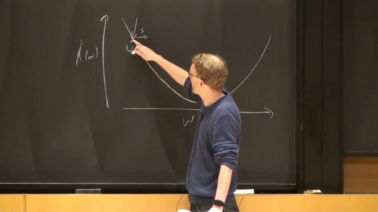
Gradient Descent & Newton's Method | Cornell CS4780 Machine Learning
@kilianweinberger698
52.8K views•2018-07-11

Secure Multiparty Computation (MPC): Foundations & Challenges
@SimonsInstitute
7.3K views•2015-05-28
Adversarial Examples & Training in Deep Learning | Stanford Lecture 16
@stanfordengineering
224.7K views•2017-08-11

Neural Networks Explained: Math, Layers, and Learning Fundamentals
@3blue1brown
21.9M views•2017-10-05
Related Study Plans & Knowledge Roadmaps
Structured learning paths in Artificial Intelligence