
















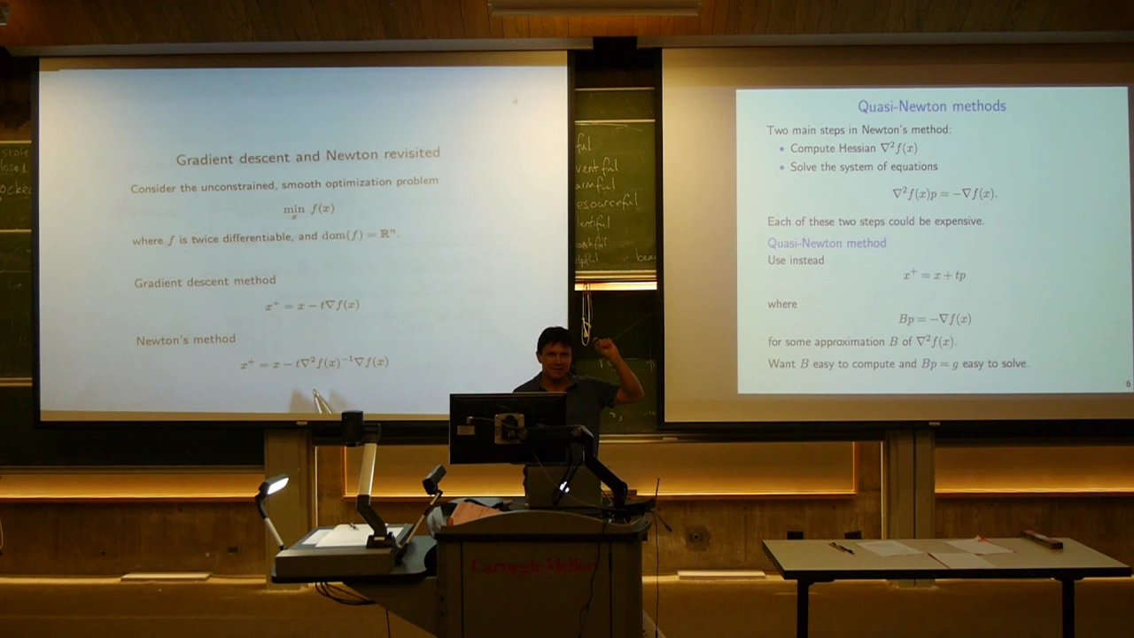




This lecture explains how to minimize loss functions in machine learning through iterative optimization methods. Gradient descent uses the negative gradient direction (w_new = w_old - α∇L(w)) to iteratively approach the minimum, with learning rate α chosen carefully to ensure convergence. Newton's method improves upon this by incorporating the Hessian matrix (second derivatives) to take larger, more direct steps toward the minimum, converging much faster once close to the optimum. However, Newton's method requires computing and inverting the Hessian, which is computationally expensive and can lead to divergence if starting far from the minimum. The recommended practical approach combines both methods: use gradient descent initially to approach the minimum reliably, then switch to Newton's method for rapid final convergence.
Gradient Descent & Newton's Method | Cornell CS4780 Machine Learning
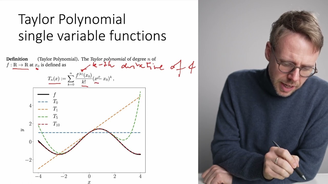
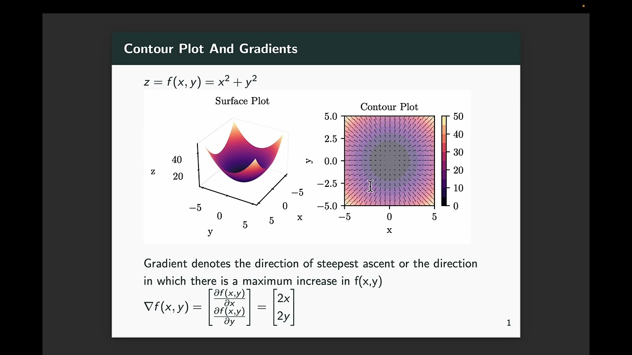
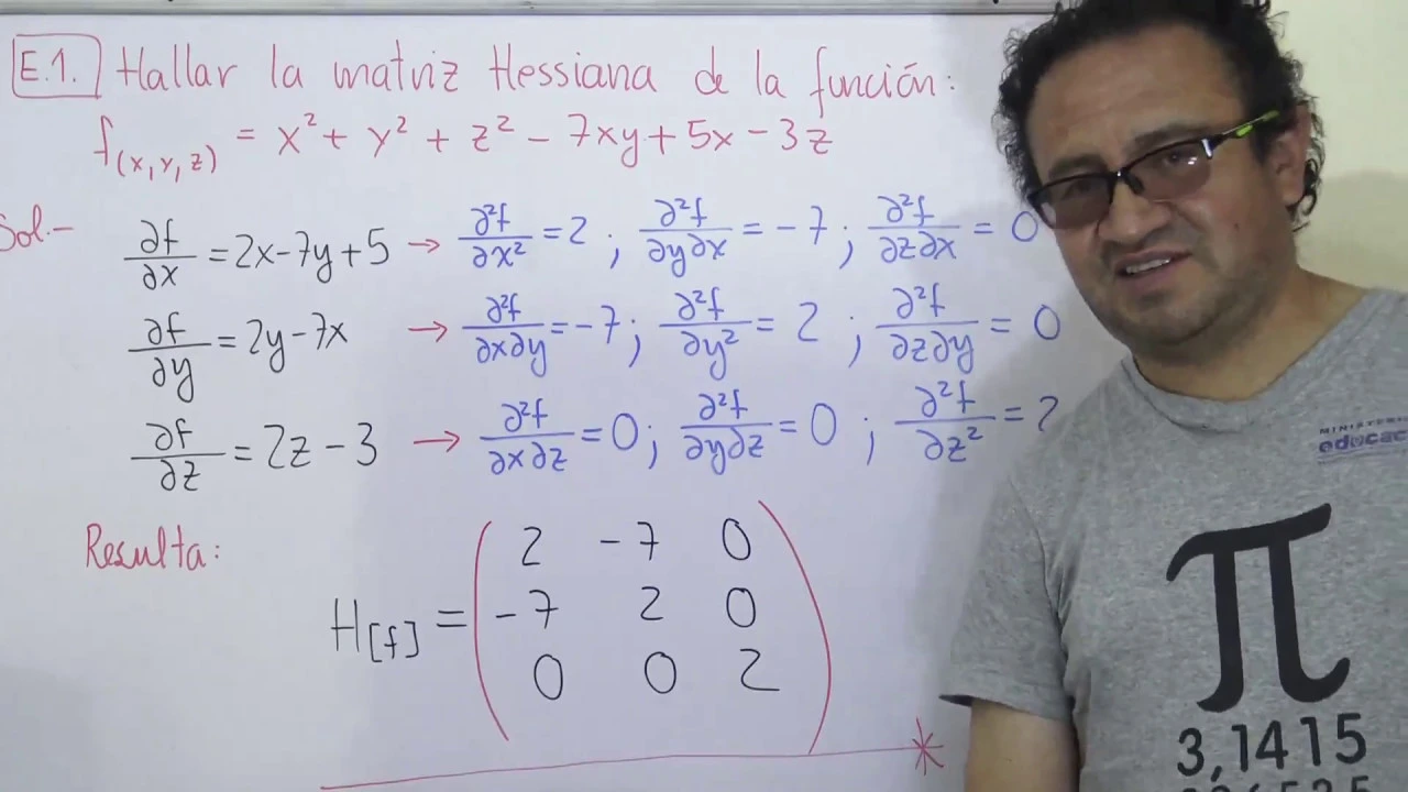
Added:all right welcome last time we talked about logistic regression [Music] thank you know I come oh thanks - neat I'm a gasping oh okay sorry about this [Music] it's not good luck I'm sorry okay so last time we talked about logistic regression and that was basically the way we derived this was by saying well what in a naive face you know learns P of X given Y and P of Y and you put this together to get P of Y given X and in order to do this tractive levy here we make the nice base assumption well turns out in certain cases this P of Y given X actually if you do nice base UK actually get a very interesting formulation you get a linear classifier in particular in you know the gaussian case which is something you will prove in the homework this will have a very specific form will have the form 1 over 1 plus e to the minus w transpose x times y and this is called a sigmoid function and so well one thing we thought is well if it has that form you know anyway why do we fit this function by actually fitting P of x and y why don't we just instead assume this form and then actually optimize the likelihood for P of Y given axis is what we really care about ultimately what we really care about is making the prediction of Y given X and so we looked into this so it's my mic on I feel like it it's not on is it on thumbs-up thumbs-down no it's not on want to test better alright okay good yeah people the mic is off or if I start speaking German let me know so it happens occasionally so let me said okay well let's do this right let's go over they decide to do maximum likelihood estimation that's basically sum of all our data try to maximize P of Y am i given X I and so we maximize the following maximized over W the product over all points P of Y given X I we took the log we did all the stuff yeah and eventually what we arrived at is a loss function that well I know it by heart actually and we somewhat want to any take log of one plus e to the minus W transpose X I Y I and that is what we want to minimize okay so we forehand whenever we minimize something we get a nice closed form solution like you know embedded map and Emily this time you to map it Emily and we arrive with something like this all right and we don't know how to continue at this point by the way please close your laptop's thank you well not all is lost so the nice thing about this that the problem is you know this function we don't really know what to do but the nice thing is this functions actually very well behaved all right it turns out it's actually continuous and it's differentiable and actually since I've even come backs so what we do it what we do is we call this scene here our last function our loss of W and so we can just view this as an abstract problem we have a function of W and we would try to find its minimum okay there's something you've done ever since high school I believe right it's basically this just you know good old analysis given a function where does it have its minimum point all right any questions at this point some people asked me some interesting questions last time that I just want to relay to everybody so I make this point to that P of Y given X is actually that's what we really want to minimize and so it's actually logistical question seems to be the better thing to do you know instead of naive Bayes right so then the obvious question is why did we spend three lectures now you're talking about naive Bayes if you should just do doing be doing logistic regression all right and actually it's not so clear-cut right it's not that logistic regression is always better than naive Bayes and the reason is quite simple when you don't have all that much data let's say you in a regime like for example you do spam filtering right well there's actually two reasons there's two reasons why you want to pay for an I face for spam filters for example the first one is an I face is really really fast you don't have to Train anything here we still have to figure out how to me to find the minimum the second thing is imagine you've only seen a couple of emails right the problem with logistic regression is you have a very very high dimensional space and you're trying to predict Y given X and this there's infinitely many hyperplanes and so essentially what it will do it will be extremely biased towards these by these few emails that you've seen right so if you're just a very few data points it will actually not give a very good classifier because it will essentially over fit and we will talk about overfitting very soon all right naive Bayes is not so prone to that and the reason is because here you make an egg out an assumption you actually you add additional knowledge right that you put in you're saying this distribution has to be gaussian and by doing this you're reducing the number of hyperplanes you could possibly learn drastically right that is that's a bad thing if you have a lot of data if you have a lot of data then why would you reduce the number of hyperplane that you can learn right just learn the best one that separates your data but if you have very very little data if you only have a couple of data points right then there's just too much degree of freedom and you're going to learn something that is you know overfits too much to these few data points then actually naive Bayes is actually much better now turns out for spam filters most people are pretty lazy and they very rarely spam is not spam and one thing you want to do is you want to give them a good spam filter right at the beginning when they tried your product for the first time right so we actually knife base texture typically what people use in this case so it's still you know it's still used very heavily it's just when you have a lot of data then actually typically to this aggression it's the way to go any questions about this no all right so here today I will post a look into this this abstract problem of saying you have a function L of W you know and I want to minimize and this is a very general thing and turns out that many machine learning algorithms not that not just with justing aggression many machine learning algorithms can be written as in exactly this form right and we call this our last function so what this basically does it it measures how many points do you get wrong right that's essentially what this function does so all right so what does this function look like I told you it's continuous differentiable and convex so it kind of looks like this is something else right so it's kind of like a like a bowl that means it's convex it doesn't have any jumps in it that means it's continuous and you can't compute the derivative so it's differentiable and we would like to find this point here right that's our target okay so the way this works is there's many many many different ways of doing this and optimization Theo is its whole own field of mathematics but I will tell you today the basic principle and essentially most algorithms don't deviate too much from that so here's the idea right what we do is we say well initially we really don't know where there's many moments we have no idea which parameter setting is the mineral right if you knew it we had a closed-form solution we'd be done we don't know so what do we do we just assign W to anything we want it doesn't matter all right whatever just make it all zero so all random varies right you know put in your own your birthdate encode it in the in the weight of W so you have now some point here which is my initial W 0 okay so basically this here's my axis and see as W in this year's the loss of tab okay so initially I just said you know my loss to anything I want it doesn't matter and so now the important thing is I would like to know which direction does this the minimum line right and so basically that he defines like some some direction that I want to walk into is call this s right and I basically want to you know identify which direction do I have to go and then I take a small step in this direction and then I get a new point and then I look again right that's the basic idea behind hill climbing in this case we're not climbing we actually tie to find the minimum so function minimization okay any questions at this point all right yeah question is there more handouts there should be more handouts I printed as I printed enough and there's a lot of empty seats who has two handouts who has more than two sorry oh this whole thing hasn't got any oh I'm sorry wait but but I'm confused are they somewhere if you know someone who has the handouts please point in that direction people people are playing if he was actually oh I'm sorry how does that way that's really bizarre I had 300 copies there's not 300 people in this room now someone leave someone leave with a big sack full of notes I'm sorry I don't know how to resolve this yeah there's nothing I can do I'm sorry alright I will guard them more carefully next time there will be online so yeah oh but then I have a mad rush at the beginning okay well I could okay I could put them in the entrance and find some algorithm okay okay good my suggestions please post them on Piazza if you have some convergence rates actually I but you know appreciate okay good all right so we have this function to minimize the problem is we don't know what this function looks like right so we know it kind of looks like this but it could be nasty right and you also don't know how much of a step you should take right if you take too much of a step then we may overcome it you know right now it looks like this but the function could also look like this right so then if you here we take a step that's too large we actually end up over here right which is not what we want or if you take a step a little bit too large view over here which is really really hard high right so how do we find this minimum and the assumption is that you know what we do is a very very simple trick as basically we say well this function is really really complicated and we don't know how to minimize it but let's just assume the function is was easy it was really simple and for example linear or quadratic and if the function was linear or quadratic we could actually find the minimum very easily right and so basically what we're doing is we we say well you know here let's just fit a line and say assume this year was in line right well if the function was just a line then it's easy to figure out a misdirection you should go right just go in the direction where it goes downhill okay and you just take a step in that direction and then you you hear you can you fit a line and you basically look at this again right so that's that's the idea more formally what we're gonna do is we're gonna use Taylor's expansions who's heard of Taylor's expansion raise your hand Oh perfect beautiful all right so take this expansion is quite simple it says you can approximate this function L by saying L plus s is roughly the function W plus the gradient at W times s right so it's like this is just this times s so what's going on okay good thank you [Music] right so basically what we're doing is we say at this point like a potato expansion by Z says is this function is continuous and it's differentiable what does that mean that once again if you're a teeny little ant you're sitting right here right what you would think is that the function is actually a straight line right if you're just small enough right because the function is smooth right if you just zoom in enough right at some point you will actually not feel the curvature anymore right and this is exactly the effect if you have planet earth right so it's globally has a huge curvature but actually if you just look here actually looks damn straight right so that's basically what we're doing here right we say locally actually this function the approximation that the function is linear is not a bad approximation and in fact this is not just the only thing you do we can actually say well we can approximate even better if you add a second derivative and then we basically say well this is plus 1/2 s transpose H of W s and cbz say what's the function value at W and then I go a little bit in direction of s if s is just small enough then it's linear right then the base is a little larger then I guess you know a better approximation actually is if I take the second term into account as well then what I'm doing essentially I'm saying the function is not just a line is actually a parabola locally right so it looks like a parabola ok any questions do people know what the age of W is if the Hessian who's heard of Hessians outside of history okay so the hessian base these are matrix that baby just says the IJ entry is the derivative with respect to well I mean let me write it down so H I J is the derivative you know of L with respect to W I and W J is actually the second derivative generalized to you know functions with multiple inputs okay and so actually tailor approximations as if you just you know you take the first derivative second derivative and the third derivative and so on you know they could eventually eventually make it arbitrarily close if the function is you know differentiable enough we will stop after first and second derivative right because the reason is the first and the second derivative these are actually if you just look at the first derivative it's a line and we know how to minimize lines and if you look at the second derivative it's a parabola and parabolas are also very very easy to minimize in fact we can do it in closed form right so those are the two these two is this approximation basically is simple enough that we would know how to minimize the function now the trick however is this approximation only holds when s is really really small right so you kind of say oh the function is roughly this that's minimize this thing on the right right and then you're done that's not gonna work right so for example if you have this you know parabola some some what you would do is you would jump here and then you would actually find the minimum here well that's obviously wrong right so the assumption only holds for small steps right so basically the way it works is we approximate the function as the Taylor expansion we minimize we take a step towards the minimization of the Taylor expansion and then we approximated again and we repeat that process and that's basically how these function minimization processes work okay any question yeah why don't you make s believe a small end well why don't we just use the linear approximation okay good question so he says this Hessian I don't like the Hessian right what have they done why don't we just use the linear approximation if s is small enough that's a sufficiently good approximation and that's actually what most people do alright there's a reason why you may occasionally want to use the head shift the reason actually is that you have to take many many many mini steps and so sometimes it's the case that you would have to take 10,000 mini steps or you take two steps for the hair shoe so it can be a lot faster right but it's not always the case and I we will get to this in a minute okay so the first gradient descent is first up is gradient descent a lot of you I'm sure I've heard of it is the most general framework of minimizing a function that's essentially exactly what you just proposed green descent basically what you're saying is the fact this this vector s that we want to add to our function to go downhill is just the negative gradient right it's just the gradient w times x times a small step size times a negative sorry so we had where is it sorry one sec ah [Music] so here we had this little picture that we Daisy have our w0 and then we take a step s and here I'm telling you a gradient descent we just say s is the gradient at W times some small learning rate and then we negate the whole thing and so why is that the right thing to do alright well if you just look at this approximation then it's very very easy to show that actually if you take this step it will always take a step down we will always reduce the function value let's just test this for a second so a loss function L of W plus s which is now this term here so plus minus alpha G of W okay so now we have our original W because I'm telling you this here is the step this is basically this this step in which we want to take from our original W and I'm claiming this year should be less than just L of W so it should be less than the value that we started from right if that's if that's true then I showed you that we by taking the step we went down here so we know that this is roughly if alpha is small you can make this as small as we want and this yes is small so we can make alpha small enough that the Taylor approximation holds then that is L of W plus this years or I guess - in this case minus alpha times G of W this is s times G of that okay so all I did here is I plugged in minus alpha times T of Java you into the s up here right and then we get this term here raising hand if you're still with me awesome and well what is that let's just look at the sine of this thing this e is the square of a rect vector so that's greater than zero right alpha if you just choose alpha to be small but positive so let's do this off as great as zero right that's a skinny parameter so that whole thing is still positive and then leave a negative so this thing here is negative right less than zero so we take we take the like the Elif double austell of W and we subtract something from it so that's clearly less than L of tavi okay so what I just showed you is that no matter where you start right no matter what you starting point W is you just compute the gradient multiplied by the small numbers and if you subtract that from your W you're taking a step downhill and so if you do this often enough you will eventually come to the minimum and so that's basically the idea right why will you eventually come to the minimum wait a second why is that guaranteed can anyone tell me yeah because the function is convex right so that's right so it could be if the function was not comebacks it could look like this right many of you start here you go down here go down here go downhill here at this point what happens here here in the stationary here that waiting to 0 right so you stop all right so you think you're you're done but actually you know this can be obviously deep here as you can connect really bad but because the function is convex and I think this was actually on the placement exam to show this you don't have to worry about this right so you keep going down keep going down keep going down and eventually you will stop why are you going to stop because at the minimum the gradient is zero right so that point you you know you basically know that you found it right you're not moving anymore okay any questions about this process No yeah how sorry how do you be alpha good I was waiting for the question that's exactly right right how do you find alpha we said alpha has to be so small the Taylor approximation holds well how are you gonna do that and well one thing is you can just err on the side robbery alpha is too small right if alphas really really small the until approximation will certainly hold the problem is then you're taking tiny tiny tiny tiny steps and it will take forever right and it may take your whole lifetime to minimize the function right so then actually it's probably much better to wait a little bit and buy faster computers in ten years and then just start then so the question is how do you find this alpha and and this is actually something that the community has thought about for a long time and I think what I when I started my PhD it was still consider the dark art and people thought well you just use voodoo right so everyone has their own kind of mechanism right now all you know eventually I start out with point one and then eventually I decrease it right and you had your secret sauce now you know fast forward a little bit it's actually very well understood so for once a really safe way of doing it is Phase II just saying alpha is some constant divided by T but T is the number of updates you've already taken if you do this then it will provably converge and the reason is no matter what your constant is in the beginning but eventually this will become so small that Taylor series holds and so you don't have to worry about it and you know you can make it can you you can make your constant large enough that it will converge eventually yeah that's not very good because it's still very very very slow in the last two three years people have actually made some sufficient progress here and I can damn it what is this is horrible okay and nowadays that people do is actually much more sophisticated and I want to want to quickly go into this it's called a de Gras oh my god and only a couple it was only invented a couple years ago but it's basically really taking the community by storm and the idea is very very simple the ideas well here's how it works right if you have a very very it depends really on what your function looks like right if your function looks like this and you're here right you want other to be very very small because alpha is too large you're gonna jump over this this thing right if you function the other hand looks like this right then you want to have alpha pretty big right because being spun pointing this direction you want to huge steps right it's not so steep and so essentially the mechanism I'm just going to explain to you as a heuristic I'm not gonna but it turns out X you can derive this very very nicely and it's very principled it is very simple what you do is as you do your optimization you keep track of the gradients that you've had in the past and the basically what you're doing is you say the following well imagine you have different features right so you have some features that are basically tracked and you know you have medical records some attract in millimeters so you hide in millimeters there's a very large numbers I don't know why you want to do this but you know and or you let me give it this better example let's say I have spam spam filter I have word counts right some birds will be very very common right like the and a and so on right these are stop words but even you know banana is gonna be much much more common than maybe hippopotamus or something right so words have different bird frequencies so what happens is that basically the gradient of Ariel across the different features right and so really there isn't really one good learning rate for every single feature so ideally for each feature you'd have a different learning rate right but now we made the problem even worse right before we just had one learning rate how do you fix this one this was a dark all right now we have to fix a thousand or maybe a million learning rates right every single dimension should have its own learning rate and so here's what I regret does it base says as we keep optimizing so hey I put in my notes that's right as you keep optimizing what we do is you have this algorithm that we say now we repeat they could be evaluate you know lfw sorry the gradient of W and G equals DL DW that's a vector right and then what we had before is we said okay G W becomes W minus alpha times G right so that's the gradient descent algorithm and we don't know how to do this alpha so here's what we do we do the following we just we start with some vector s which is initially is zero we put our for loop and then every time you complete a gradient we say s becomes s plus G squared and can you explain what I mean by this where the Julia people I think every single energy is squared okay so you can either write this as this so you know so or you can write it as this G all right so lazy you just take every single entry and square them but you keep it a vector you don't sum over them okay so it's not G transpose G is G dot star G so what you're doing is you be easy to keep track of on you know an average a like home how large the gradient walls and past's in past steps and then what are you doing is you take the grain that you have an element-wise you divided by the square root of the Sun plus some Epsilon so essentially what this means is when in the past I had a feature where the Grady was very very large right then this is very very large right because I square it and I sum over all the different changes so that means if I divide the gradient by it the steps that's going to be really small all right so if I very steep and some feature them in some dimensions I will have very steep surfaces and for those that take small steps in other dimensions I have very shallow surfaces I take large steps okay and that has really become kind of the beauty of it is you still have some some constant here that you can set but doesn't really matter you can just set it to one and then you just get rid of it right ultimately it sets itself right so busy takes past gradients and it learns how to set the learning rate any question yeah oh oh I'm sorry is that true oh I see Oh OSI does my notes are wrong actually right OSE in the nose that should be SS instead of GS I and then there's notes I call it I call this s and this SS which I blame on momentarily insanity okay any any more questions yeah Paul why's Epsilon oh it's just because in case something is zero imagine you have some feature we just have no gradient ever right that also means that feature doesn't matter right but that means s squared would be zero and you would be divided by zero and everything would blow up so you just add some constant to it and then you get a very large learning way that probably doesn't matter because then rate is zero right yeah good I mean in some sense because you just added this write the gradient must be zero here so it doesn't actually matter what you do in that case right good question yes any more question so X are just ten to the minus five or something oh yeah the very back yeah [Music] oh good good good right so so the question was well actually we're just getting closer and closer and closer and as we get really really close to the minimum what's gonna happen the gradients gonna come you know go become zero right here the zero so here it's gonna become really really really small right so what will happen we actually take really really small steps so when we actually ever really get there right so when should we stop this whole whole algorithm and so you do exactly this you basically keep track you say this here's my T plus one this here's my T and you say you stop if you know if the norm between T plus one minus WT is less than some some small Delta then you break then you stop right so usually always have some color please say if my weights have not changed the last round then I'm stopping right the important thing is there's really something that people didn't realize for a long time it's enough people use these concepts of optimization for your mathematics and optimization theory they're really concerned of getting exactly to the minimum by accuracy up to ten to the minus ten or something in machine learning we don't care about this right because ultimately what we want to minimize essentially is just the zero one loss right leg end you just want to have good predictions and if you get a little bit closer probably doesn't make any difference right so you know this Delta can be sufficiently large okay any more questions okay good so that was grading descent now come in the Hessians so great nice and it's really nice the only thing is and there's actually the step that you said it's really nice getting close to the minimum but once once you're in Lewisville inity it slows down so the the most of its time almost all its time it will spend you know nose to the minimum okay because that's when the gradient is small so the question is can be vitas apps like once we are close to the minimum 10 we get right to the minimum you know up to some Delta that we can stop and this is exactly where the the second order approximation all right so so far what we said is you know we just approximate there's a lion amazing step you take a step in direction off this line the slope now we're basically going to take a parabola and so seconds so the idea is quite simple you can just say exactly this function here and just minimize it with respect to s we say wait Taylor's approximation tells us our function is approximately this way now don't cross this out any what kind of just minimize this there's a quadratic function and what's exactly the step size that I would have to take to minimize this function so what I'm saying is I have some W here I find this parabola now I pretend my function really is the parabola and parabola sickens minimizing closed form so I can just find the minimum of the parabola right that's what I'm on so forth and this here is my X further the the difference from W that I have to add to get right to the minimum of the parabola and once I'm here that I again fit a parabola I find a minimum again I fit a parabola and then I'm done Newton's method converges superfast blazingly fast I just need a couple of steps like if you take 10 Newton steps you know you're you're you know you're gonna be the absolute you know a numerical accuracy usually when you have low low accuracy numbers I get machine learning a few Newton steps typically get you there very very quickly so let's just quickly do this so you want to minimize this respect to s so minimize this function with respect to s and what do we do what do I do when I minimize a quadratic function it starts with gray and ends with the end I think someone's that a gradient it's like a few the gradients it's back to s this here zero this is g fw this year is now I have to take matrix gradients if you're not familiar with matrix gradient look at the matrix cookbook I think I'll link to it from my from the home page as that's H of W times s and you want to set this to zero so this here is the gradient of this function with respect to s that's zero what do we do well it's quite simple right so we just put this on the other side so s equals G of W minus 2 u fw and to get this function this matrix over there we just take the inverse right H of W inverse nice we divide by this that's what you have to do so Newton's method what you do is you just take your random vector W you compute the gradient and you compute the hash stream and you multiply the gradient with the inverse Hessian and that's what you add to your function and that basically gets you down really really really really quickly so Newton's method is awesome there's our one dance there's one downside and this downside is most of the time it doesn't work at all so most of the time what happens is that when you when you have a function that's really really flat right what you're now doing is you're approximating that with a parabola and that parabola could look like this or something like this and now you're taking a really large step that's every function looks like this something now you take a really large step right this here's my s and if you take reading our steps Taylor approximation doesn't hold anymore right and so what you're doing is you're shooting off into no-man's land right all right let me give you an even better example let's say have a really any function like this right function like this this is my convex function right so it could very well be that my parabola that I'm using here looks like this right approximating this way so I start here I jump all the way here to that minimum all right now I end up here right not approximated again with a parabola and I end up here right and I'm spiraling out of control in no time so Newton's method really only works if you're very very close to the minimum already nice and your function is not well I show you some examples why not show you some examples so the best typically what I recommend people to do is to Grady descent for a while and then just before you end take two or three Newton steps right and then you're basically then you sort it right because then you have basically at the minimum any questions well people buy that I also do is they sometimes just take the diagonal of the Hessian that also works reasonably well those are called second-order methods or there's conjugate gradient that approximates it yeah well in some sense you're solving for the whole thing right so it's no longer if you don't scale it I think you still wouldn't get any little convergence guarantees actually in some sense the benefit would be gone what is this does not mean all right okay good all right so here's a how much time you have okay and so first I just want to show you a little so okay so first a little example of just good old Grady descent so here's my function and the red point is where I initialized it and the middle is actually control a function so that the minimum was actually here at zero right and so now I can be put on the different different step sizes and see how long it takes me to converge right and so the first thing I can do is I can just set the step size to find one all right and now you can see the different steps I know if you can see these can you see them it basically takes all these these red lines here from here to here basically is a step right so all these different things so I took all the way eighty-three steps right so took eighty three steps to go from here to here and then it basically converged up to some Delta I can do the whole thing again with a smaller step size then actually it never converges at some point I just said maximum number of iterations has reached so I never get there right if I make my step size larger let's say I just do you know five right why not then what happens this happens right so here's my function weight and this year busy you see this here's my function out here and this is kind of Jupiter and this is you know like Neptune or something be way out there in outer space right oh my gosh come on where is it I see something I'm hopeful [Music] all right so I'm really really out there all right so you get the point sorry oh yeah central 195 great yeah that's more than electrons in the universe right so we are really really out there right so I didn't even take my step size that large right I was just a little bit lighter right and be have rights did I shoot past the minimum all right so setting the step size is important I can also show you some Newton steps so here she had the demo1 Newton so here's another example there's a beautiful function and now Newton the beautiful thing about Newton's method I don't have any step sizes to choose from right so I can just you know I just run it and I converge so we can first say okay well let me just start at 0.3 right and at 0.3 my conversions nice steps right well I'm pretty accurate here very very accurate if I you know say you know let's say I or this is all point three I start up here okay that's pretty steep so if I started you know whatever it's two right then I would only take eight steps and I'm actually here right and the nice thing is every single step you X usually get one digit off of significance of accuracy what if I start at nine right and so that means I'm starting over here and I do my Newton search right then BAM right what happens well I'm actually oh and I'm still fine wait I'm still fine this is amazing okay let's do seven that's 210 okay now I diverse right so now actually if you zoom out if I try to zoom out which I can't so one thing you can see wet is the red line actually okay I can't zoom out I'm sorry I don't know what happened basically I'm again in outer space right so the difference is the Newton step the equivalents in some sense like gradient descent you have to set a step size right Newton said only works at certain starting points right the good news is you can check very easily if you made a mistake right if you're lost and suddenly a lot larger than you know oops right Newton step doesn't work here yet just keep doing a few more gradient steps alright I get using the same thing one more time in 2d now Simon's over ah shoot here we go here we go so what you can see here is actually a function that I'm trying to minimize alright so so what you can see here is basically the black line is basically gradient descent here's my function at this basic function value this number of steps I'm taking and what do you see is the gradient sent very quickly gets close to the minimum right but then takes forever to do this little last little bit right to get from here to here right takes a hundred steps right so that's exactly the problem with gradient descent right so you get close to the minimum relatively quickly but then just takes forever to finally get there all right so Newton steps actually is very very good right in just a couple steps actually it's really at the minimum if you look at the the plot here on the right jex you can see this is the function here's where I started so gradient descent takes these sorry greenie sense green ones that actually takes one step here and over and over and over you know them very quickly it's actually close but then here it actually takes forever right whereas Newton steps actually very consistently gets towards the minimum and then you can sue in any further Newton step basically just takes two from here one more step whereas the grading is sent here probably takes 90 more steps right so if you're close to the minimum you want to take this method let me do one last one before you guys leave does the here's basically if I started at a bad point so here's the same function and again you see here I'm actually the red line is Newton steps so I my function is down here and very quickly in outer space right I basically completely blew it and what happens I just started as you know so here's what Newton step does right so grading descent very nicely goes to the minimum when Newton steps like oh my gosh right like it's like so what do you do in such cases and the answer is you just take a few steps with gradient descent and then you do Newton steps right so here's what I did I took took a couple steps of gradient descent and then I switched over to Newton and then I'm okay again all right so please remember this the main take-home point when you do gradient descent to adaptive gradient to the other grad and when you get close to the minimum so maybe after you know a couple hundred steps or 1000 hundred steps switch over to Newton's method then you converge in no time
Up Next

Optimizers in Deep Learning: SGD, RMSProp, and Adam
@nptel-indianinstituteofsci8064
106 views•2026-03-20

Secure Multiparty Computation (MPC): Foundations & Challenges
@SimonsInstitute
7.3K views•2015-05-28

Bypassing Tor Censorship: Bridges and Pluggable Transport Guide
@Coding_ForEveryone
397 views•2024-06-11

Neural Networks Explained: Math, Layers, and Learning Fundamentals
@3blue1brown
21.9M views•2017-10-05
Related Study Plans & Knowledge Roadmaps
Structured learning paths in Artificial Intelligence