















![[에이플러스] 미적분학 CH25-9 (다변수) 테일러 급수](https://i.ytimg.com/vi/dQthP_38_us/maxresdefault.jpg)


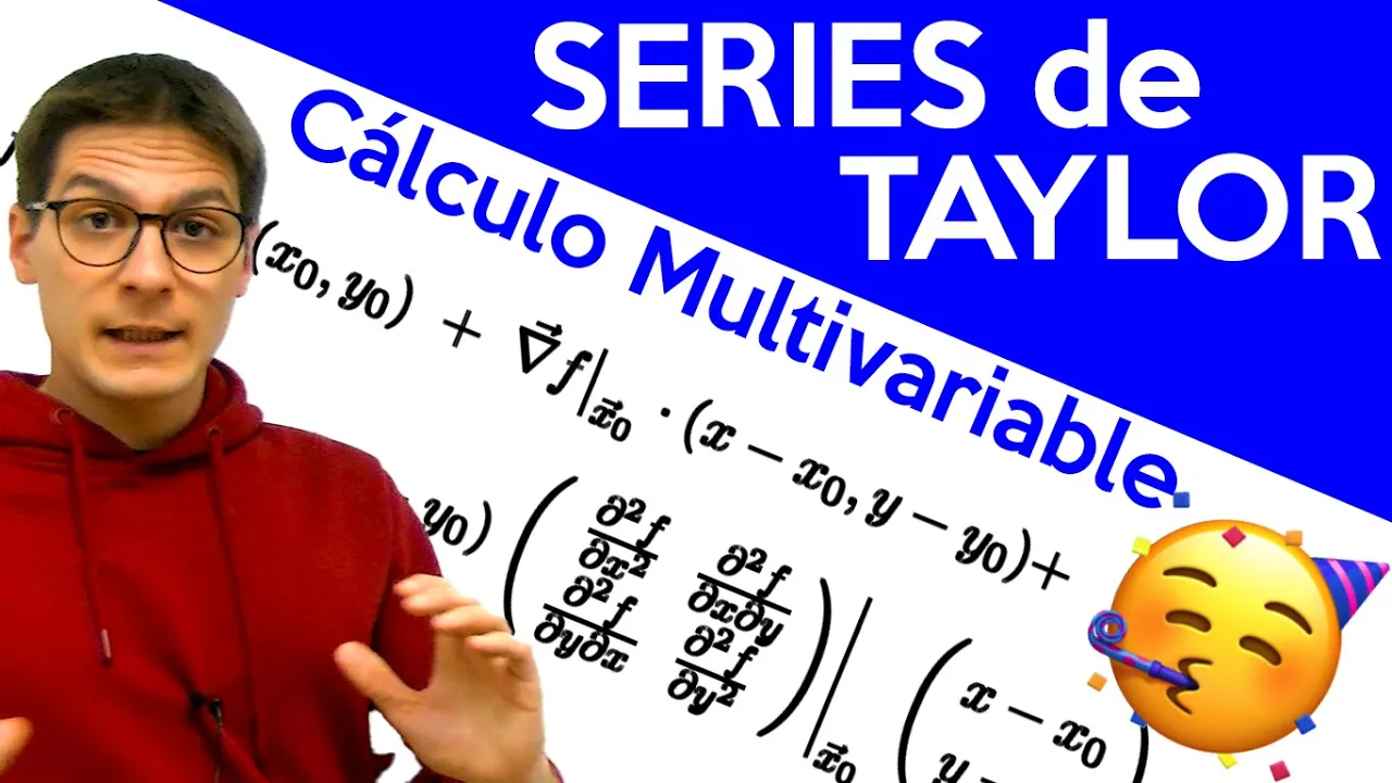

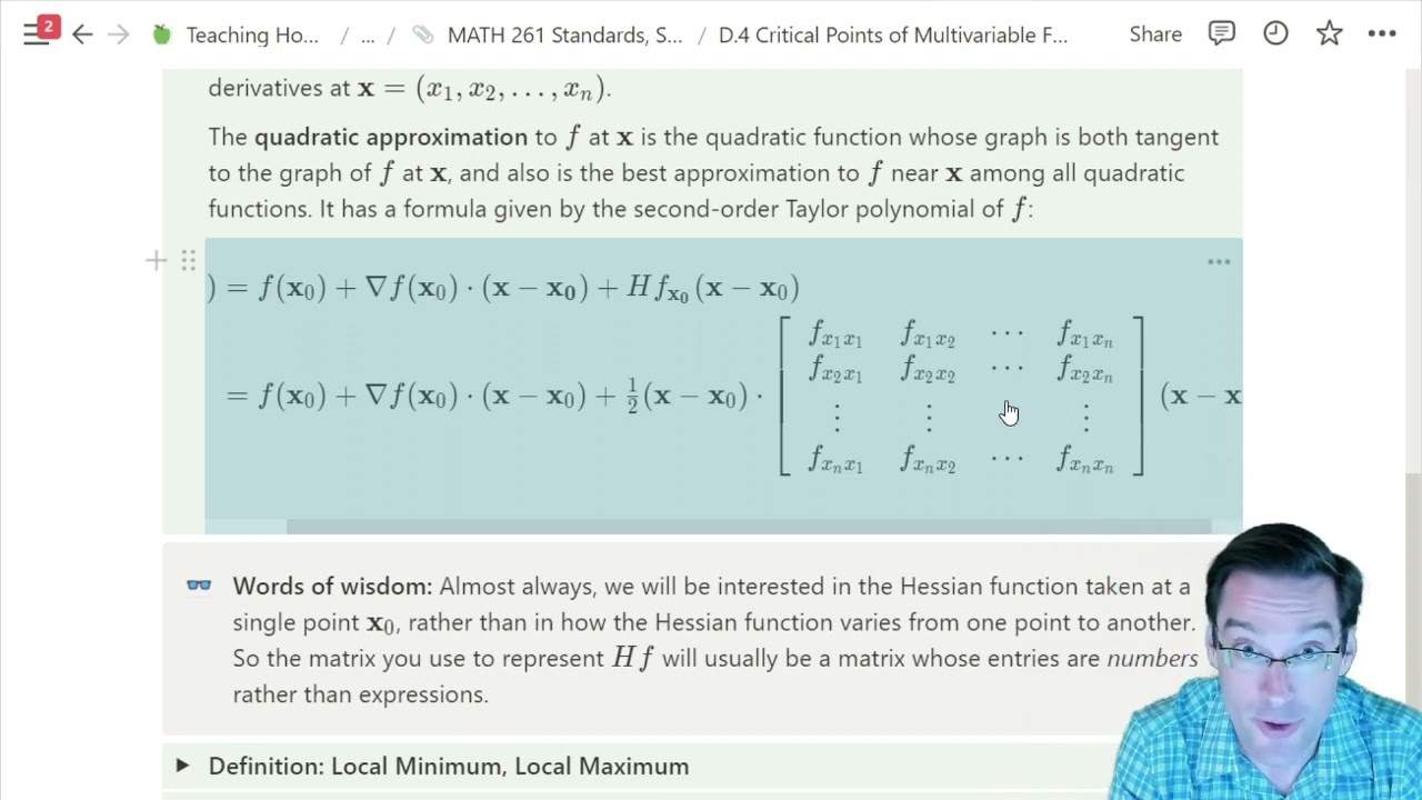
The Hessian matrix is a square matrix that organizes all the second partial derivatives of a multivariable function, where each entry H_ij represents the second partial derivative obtained by first differentiating with respect to variable j and then with respect to variable i; for most well-behaved functions, the mixed partial derivatives are symmetric (H_ij = H_ji), and this matrix structure extends naturally to functions with any number of variables, making it a powerful tool for expressing quadratic approximations and performing matrix operations in multivariable calculus.
Hessian Matrix | Multivariable Calculus | Khan Academy
Added:First-order partial derivatives and how to construct the gradient vector of a multivariable function.
Concept and computation of second-order partial derivatives, including mixed partial derivatives and Clairaut's theorem.
Basic linear algebra, particularly matrix representation, vectors, and matrix-vector multiplication.
Single-variable Taylor series, specifically the role of the first and second derivatives in linear and quadratic approximations.
The Multivariable Second Derivative Test to classify local extrema (maxima, minima, and saddle points) of multivariable functions.
Determining matrix definiteness (positive definite, negative definite, indefinite) through the eigenvalues or determinants of the Hessian matrix.
Multivariable Taylor series expansions to higher-degree polynomial approximations.
Optimization algorithms in machine learning and data science, such as Newton's Method, which utilize the inverse of the Hessian matrix.
515.1K views4.6Klikes6:10Original Release: 2016-06-16
hey guys so before talking about the vector form for the quadratic approximation of multivariable functions uh I've got to introduce this thing called The hessen Matrix hessen Matrix and essentially what this is it's just a way to package all the information of the second derivatives of a function so let's say you have some kind of multivariable function uh like I don't know like the example we had in the last video e to the X haves multiplied s of Y so some kind of multi iable function what the hessen Matrix is and it's often denoted with an H or kind of a bold-faced h um is it's a matrix incidentally enough that contains all the second partial derivatives of f so the first component is going to be the partial derivative of f with respect to X kind of twice in a row and everything in this First Column it's kind of like you first do it with respect to X um because the next part is the second derivative where first you do it with respect to X and then you do it with respect to Y so those that's kind of the First Column of the Matrix and then up here it's the partial derivative where first you do it with respect to Y and then you do it with respect to X and then over here it's where you do it with respect to Y both times in a row so partial with respect to Y both times in a row so let's go ahead and actually compute this and think about what this would look like in the case of our specific function here uh so in order to get all the second partial derivative we first should just kind of keep a record of the first partial derivatives so the partial derivative of f with respect to x uh the only place X shows up is in this e to the X Hales kind of bring down that 1/2 e to the X Hales and S of Y just looks like a constant as far as X is concerned s of Y and then the partial derivative with respect to Y partial derivative of f with respect to Y now e to the X haves looks like a constant and it's being multiplied by something that has a y Y in it e to the X haves um and the derivative of s of Y since we're doing it with respect to Y is cosine of Y cosine of Y uh so these terms won't be included in the Hess itself but we're kind of just kind of keeping a record of them because now when we go into fill in The Matrix this upper left component we're taking the second partial derivative where we do it with respect to X then X again so up here's up here's when we did it with respect to X if we did it with respect to X again we kind of bring down another half so that becomes 1/4 by e to the X Hales and that s of Y just still looks like a constant s of Y and then this mixed partial derivative where we do it with respect to X then y so we did it with respect to X here when we differentiate this with respect to y the2 e to the X Hales just looks like a constant but then derivative of s of Y ends up as cosine of Y and then up here uh it's going to be the same thing but let's kind of see how when you do it in the other direction when you do it first with respect to Y then X so over here we did it first with respect to Y if we took this derivative with respect to X you'd have the half would come down so that would be 12 e to the X haves multiplied by cosine of Y because that just looks like a constant since we're doing it with respect to X the second time so that would be cosine of Y and uh it shouldn't feel like a surprise that both of these terms turn out to be the same with most functions that's the case technically not all functions you can come up with some uh crazy things where this won't be symmetric where you'll have different terms than the diagonal but for the most part those you can kind of expect to be the same uh and then this last term here where we do it with respect to Y twice we now think of taking the derivative of this whole term with respect to Y that e to the xav looks like a constant and derivative of cosine is negative s negative s of Y so this whole thing a matrix each of whose components is a multivariable function is the hessen this is the hessen of F and sometimes people will write it as hessen of f kind of specifying what function it's of and you could think of this I mean you could think of it as a matrix valued function which feels kind of weird but you you know you plug in two different values X and Y and you'll get a matrix so it's this Matrix valued function and the nice thing about writing it like this is that you could actually extend it so that rather than just for functions that have two variables let's say you had a function I'll kind of like clear this up let's say you had a function that had three variables or four variables or kind of any number so let's say it was you know a function of X Y and Z then you can follow this pattern and uh following down the First Column here the next term that you would get would be the second partial derivative of f where first you do it with respect to X and then you do it with respect to Z and then over here it would be the the second partial derivative of f where first you did it with respect to uh first you did it with respect to Y and then you do it with respect to Z I'll C clear up even more room here uh because you'd have another column where you'd have the second partial derivative where this time everything you know first you do it with respect to Z and then with respect to X and then over here you'd have the second partial derivative uh where first you do it with respect to Z and then with respect to Y and then as the very last component you'd have the second partial derivative where first you do it with respect to well I guess you do it with respect to z twice so this whole thing this 3x3 Matrix would be the Hess of a three variable function and you can see how you could extend this pattern where if it was a four variable function You' get a 4x4 Matrix of all of the possible second partial derivatives and if it was a 100 variable function you would have a 100 by 100 Matrix so the nice thing about having this is then we can we can talk about that by just referencing the symbol and we'll see in the next video how this makes it very nice to express for example the quadratic approximation of any kind of multivariable function not just a two variable function and the symbols don't get way out of hand because you don't have to reference each one of these individual components you can just reference The Matrix as a whole and start doing Matrix operations um and I will see you in that next video
Up Next
8:53
Understanding the Jacobian Determinant and Its Geometric Meaning | Multivariable Calculus
@khanacademy
229.7K views•2017-01-10

4:43
Elliptic Curve Cryptography Explained: ECC, ECDSA, ECDH
@PracticalNetworking
28.5K views•2024-10-21
6:22
Jacobian Matrix Explained | Local Linearity & Transformations
@khanacademy
580.9K views•2017-01-10

6:00
The Mathematical Impossibility of Accurate World Maps
@Vox
23.3M views•2016-12-02
Related Study Plans & Knowledge Roadmaps
Structured learning paths in Mathematics
mathematics
Tensor Calculus: Vectors to Riemann Curvature
01Mathematical Foundations: Linear Algebra & Calculus
02Covectors, Dual Spaces, and Tensor Basics
03The Metric Tensor and Index Gymnastics
+ 2 more learning modules
40h5 modules
Explore Roadmap
mathematics
Gödel's Incompleteness: Logic, Proofs & Limits
01Introduction to Formal Systems & Hilbert's Dream
02Set Theory, Cardinality, and Cantor's Diagonal Argument
03Arithmetization and Gödel Numbering
+ 2 more learning modules
14h5 modules
Explore Roadmap
mathematics
Galois Theory: Fields, Groups & Solvability
01Foundations of Abstract Algebra: Groups & Fields
02Polynomials & Field Extensions
03Splitting Fields & Symmetries
+ 2 more learning modules
24h5 modules
Explore Roadmap
mathematics
Non-Euclidean Geometry: Models & Geodesics
01Euclid's Fifth Postulate and the Birth of New Geometries
02Hyperbolic Space and the Poincaré Disk Model
03Geodesics: Defining Straight Lines in Curved Spaces
+ 2 more learning modules
15h5 modules
Explore Roadmap