




![BACKPROPAGATION [MACHINE LEARNING]](https://i.ytimg.com/vi/AE6QvdmUQ0Y/maxresdefault.jpg)
















This lecture explains adaptive learning rate optimization methods for training neural networks, including SGD with momentum (which uses an exponential moving average of gradients), RMSProp (which scales gradients by the inverse square root of accumulated squared gradients), and Adam (which combines both momentum and RMSProp principles). The lecture emphasizes that in high-dimensional non-convex optimization problems common in neural networks, gradient descent rarely reaches global optima, making adaptive optimizers essential for practical training. Adam has become the go-to optimizer in modern deep learning due to its empirical effectiveness across various architectures.
Optimizers in Deep Learning: SGD, RMSProp, and Adam
Added:Fundamental concept of Gradient Descent, including how a loss function is minimized.
Basic understanding of Neural Network architecture and the Backpropagation algorithm.
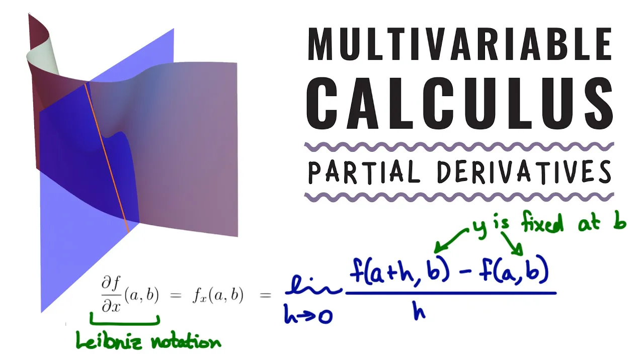
Multivariable Calculus concepts, specifically partial derivatives and the gradient vector.
The role of the Learning Rate hyperparameter and the challenges of manual tuning, such as overshooting or slow convergence.
Advanced optimizer variants such as AdamW (decoupled weight decay) and AdaBelief.
Learning Rate Scheduling techniques, including Cosine Annealing and One-Cycle policies, to dynamically adjust rates during training.
Hyperparameter optimization strategies for tuning optimizer-specific parameters like beta coefficients and epsilon.
The practical implications of batch size on optimization stability, convergence speed, and generalization capability.
106 views5likes19:28Original Release: 2026-03-20
Welcome back. Training neural networks with adaptive learning rate.
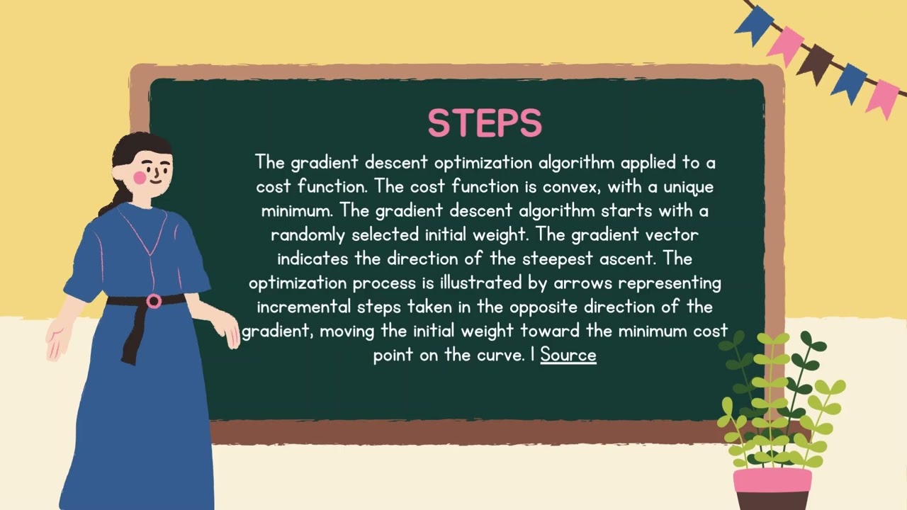
Okay. Now, neural networks are trained using erm gradient descent.
Now if uh suppose um rcap of theta is the empirical risk.
Now gradient descent estimates the parameters as follows. Now you have uh theta t + 1 to be theta t minus alpha * the gradient of the empirical risk with respect to theta.
Right? This is what the first order gradient descent is all about. Uh there are versions to it. Right? One version is what is called as the stoastic gradient descent.
where compute uh r tilda of theta as estimate the loss on on a set of samples, right? Which is uh where where B is a subset of the data set D randomly sampled.
We already saw that this has a regularization effect is what I told you. So this is called stoastic gradient descent or SGD where if you have thousand samples you construct a batch of 32 samples or 64 samples which is again a hyperparameter and then perform the gradient descent and one full um walk through the entire training data is called an epoch during training. Okay, an iteration is where you do one forward pass and one backward pass through uh the neural network that you are training. If you do a stoastic gradient descent and uh pass through the entire data set once then it's called an epoch and training is done for several epochs.
That's how the training is done. Okay, this is stoastic gradient descent. Uh but in in both in stoastic gradient descent and the gradient descent, right, the step size, okay, alpha is fixed.
This is also called learning rate.
This learning rate is fixed in stoastic gradient descent. You fix it to a particular value. Okay. And you keep it the same. But uh in optimization we know that while we are looking at uh gradient descent or rather numerical algorithms we may have to take a larger step at times where the gradient has uh uh larger magnitude and you are near the uh the optima we have to take a smaller step uh at other times and so on. So basically instead of having the fixed learning rate, it's always a better idea to have adaptive learning rate. The learning rate that adapts. Okay. So there are techniques that would incorporate this. There are a few adaptive learning rate techniques for gradient descent.
we look at uh uh a few famous uh such things. Uh the first thing is called um SGD with momentum where the idea is as follows. Define momentum mt as beta 1 * mt - 1 + 1 - beta 1 * gt where so gt is the gradient of the loss function.
And now you make theta t + 1 as theta t minus some alpha * mt.
Yeah. What is this doing?
This MT is a running average of the gradients, moving average of the gradients at t= 1. It is simply the gradient.
Okay. At when you initialize mt m0 to zero, so it's equal to the gradient. As you keep moving in time, the m the the m term will keep accumulating the gradients and taking an average of it as we move on.
Okay. Now, instead of subtracting the the the gradients, you subtract the accumulated gradients over time. Why is this a good idea?
You're computing the exponential decaying average of gradients?
Which means in earlier times you take larger steps depending upon the gradients and the later steps you take smaller steps. the the gradient because the gradients are being accumulated over time.
So this is called SGD with momentum and this term MT is called the momentum term.
Okay. The see here what did we do is that we accumulated the gradients but we know that in optimization uh the first order gradients are not enough right? you need to accumulate the second order terms of the gradients as well.
Why? Gives you the acceleration effect.
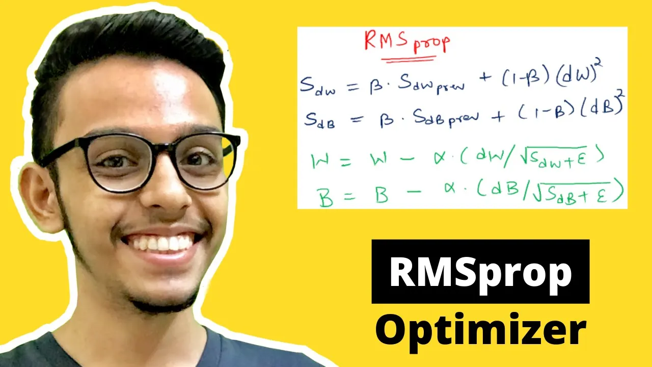
Right? So instead of only looking at the first order gradients or rather uh the gradients, look at the gradient squared terms as well. Okay? So this is called there's another adaptive learning rate method which is called RMS prop.
So here instead of averaging the gradient you average the second order or rather the squared of the gradient define wt to be some beta 2 * vt - 1 + 1 - beta 2 * gt² we are accumulating the square root of gradients here now you make theta t + 1 to be theta t minus some alpha divided by roo<unk> of v_t into gt.
So why do we need this root of wt? V_t the dimensions of the v_t and not the dimensions r dimensions it's the physical dimensions of gt is square root of gradients right. So root of wt has the dimensions as that of gradients and gt is gradients they both cancel and the one that this will be of dimensions of the parameters and that's why you can add and subtract them the dimensionality has to match right yeah so that's why this is the uh the rms prop where what we are doing is that instead of using the first order gradients or rather the the gradients we're using the gradient squared terms Okay, why do we have to do this?
See, we are scaling the gradients. All gradients are now being scaled with a particular value. This particular value is inverse of their squared.
So the gradients, okay, are the parameters for which the gradients are damping uh higher the gradients, they dampen quicker.
The lower the gradient values they they dampen slower. So here what we did was we dampened all the gradients no matter what their the so-called acceleration is. Here they are being scaled by the inverse of the uh damping factor or the acceleration. That's it.
Okay. This is about RMS prop. Uh the other update to this improvisation of this is what is called as adaptive momentum estimation also known as Adam.
And by the way, even though I've written it this way, right? Uh if theta are vectors, these are done at the element level, the parameter level. I mean these things are actually the hadamar products because when you take the square root of gradient, you you do it dimension wise.
Each of the dimension has to be multiplied. So you please note that if you do this then there there is a different learning rate for different parameter also.
You understand there is adaptability across different parameters. You know some parameters are are updated faster or larger and some parameters are adapt are are are changed slower because this is happening at the parameter level because these are vectors. No, we are looking at haramat products here. Do you see that?
Okay. So, this adaptive momentum estimation which is referred to as Adam actually combines both. It's a combination of both the RMS prop and the HTD momentum. There we have both the terms. So compute momentum as beta 1 * mtus 1 + 1 - beta 1 * gt and uh beta 2 * vt - 1 + 1 - beta 2 * gt² and the final estimate Right.
Theta t + 1 is theta t minus alpha divided by roo<unk> of v_t times the momentum.
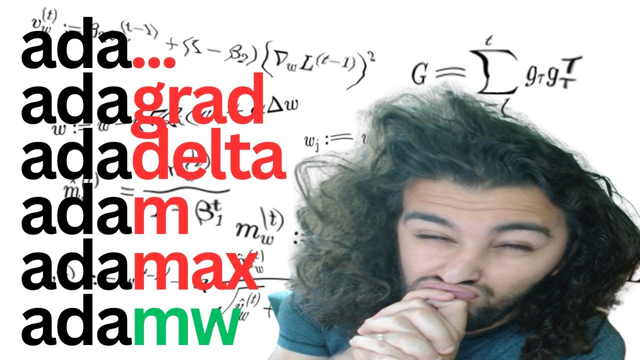
So this is a combination of both the rms prop and uh the momentum term. You have both the momentum and the second order term. This is called atom. Now if you go to the standard optimizers such as pyarch etc. you have the uh the facility to choose your optimizer. You can choose SGD, you can choose RMS prop, you can choose SGD with momentum or atom. Adam is the go-to choice for optimizers in today's uh learning because empirically it has been observed to be uh leading to good convergence. Now you have to choose this beta 1 and beta 2. They are hyperparameters.
Okay, adaptive momentum estimation. Uh, now that we are talking about uh optimizing neural networks, there is one point that I would uh I would make uh which is which is uh better to be known.
See, we are using gradient descent here.
Okay. To optimize over the parameters parameter space that would be typically a very large size, right? I mean today they are of billions of parameters you know there can be thousands of so we are optimizing in a very large dimensional space and the objective function that we are that is being optimized is not a convex function of these parameters.
The empirical risk that we are optimizing is no uh convex function.
Okay. So first order gradient descent does not guarantee that that you will go to the true optima in in fact it can be is that the the the likelihood of these methods taking you to uh the true minimizer is very very low and it can be shown mathematically. Let me just tell you that.
So let's say that we are operating in a thousand dimensional space.
Our neural network has thousand per thousand is nothing. You know a simple uh ant level MLP will also have thousand par more than thousand parameters. Let's say that you have a neural network that has thousand parameters.
Now suppose uh there is an optimization surface. When do you know or how do you find out whether a given point on this optimization surface is a point of extrema or not?
Recall your uh high school or uh college math. How gradient has to be zero.
Right? That will only tell you that the gradient vanishes at that point. How do you know that if it's a maximum or a minima?
Second derivative test. You'll have to always look at the second derivative test. Now if you are working with uh vector valued functions what is the equivalent of the second derivative test?
>> Not the hessian. Hessian is the equivalent to second derivative. But if if a point has to be a global optima then the signs of the igon values of the hessian matrix are all have to be of the same sign. If all of them are positive or in in in other words if the hessian matrix is positive definite then that particular point is a minima or maxima >> yeah whatever right it has to be it has to be all the values have to be of the exact same sign now let's say that we are operating in a thousand dimensional space what is the size of the hashian >> which is 10 to six a million we have We are looking at a million uh >> igon values. Looking at million values.
Let's say that we model the sign of the igon value as a bernoli random variable with success probability p.
What am I saying? With probability p the sign of the igon value of the hashian matrix is positive. with probability 1 minus P. The success probability is that the probability that the sign of the igon value of the H matrix is negative is 1 minus P. So now take this P to be.99999.
So with a very high probability the value of the session matrix is going to be positive.
Now what is.99 to the power of 10 to the 6?
No.99 to the^ of 10 to 6 is a very very small number right which means that the odds of any point that you land on to on the loss surface in a thousand dimensional space being a global optima is extremely low.
This by this with an assumption that the probability of uh it taking a positive value is.99.
So what am I trying to say? So now we are looking at not at thousand parameter neural networks. We are looking at millions and billions of parameters of neural network. So almost always gradient descent will not take you to the point that is a global optima. Then what is the hope? The hope is look at your validation data. The only question that all the points that we land uh to with gradient descent are local optimas.
The only question that is to be asked is is your local optima better than my local optima.
And how do we measure this? By looking at validation data. That's why when you try neural networks, there is no theoretical way to look at what the stopping criteria is.
Okay. Just you have that is why people look at come up with benchmarks. You have test data. Whatever neural network you train in performance or rather uh extract its performance on test data and that's that's your uh truth that's it okay in fact there is one other nomure that is used when you are doing gradient descent right every single point of gradient descent will give you a different model because you are navigating in the theta space correct and these things are called checkpoints by the way so what is shipped are checkpoints model checkpoints A model checkpoint is nothing but a particular set of theta for this architecture. So when you download a model a pre-trained model from some of these uh commercially available uh libraries hugging face for instance what they actually give you are these thetas with an erm done on a particular task start from it either do inference on it or you can initialize another neural network with that and you know you do another erm on top of it or do distillation or do whatever you want is okay so I think now we are in a position to take up a data set take any neural network and train it to for whatever task you want. This is the foundational principle of training any uh you know neural network for any task including LLMs and today's LLMs are trained on thousands of uh or not thousands hundreds of thousands of GPU cards for several tens of months on trillions of tokens of data that's the scale >> with billions of parameters exactly right that is what it is Right. Okay. So this completes our discussion on neural networks. We will next go to uh the class classification and regression trees, decision trees and subsequently we look at ensemble methods. Thank you.
Up Next

11:54
Q-Learning Explained: A Guide to Reinforcement Learning Basics
@CodeEmporium
82.4K views•2023-11-07

57:48
Secure Multiparty Computation (MPC): Foundations & Challenges
@SimonsInstitute
7.3K views•2015-05-28

13:03
Bypassing Tor Censorship: Bridges and Pluggable Transport Guide
@Coding_ForEveryone
397 views•2024-06-11

18:41
Neural Networks Explained: Math, Layers, and Learning Fundamentals
@3blue1brown
21.9M views•2017-10-05
Related Study Plans & Knowledge Roadmaps
Structured learning paths in Artificial Intelligence
artificial-intelligence
Aligning LLMs: DPO, TRL & Custom Datasets
01Foundations of Python & Machine Learning
02Transformers and Large Language Models (LLMs)
03Aligning LLMs: SFT and RLHF
+ 3 more learning modules
24h6 modules
Explore Roadmap
artificial-intelligence
Federated Learning: PyTorch, Flower & Privacy
01Python & Machine Learning Foundations
02Deep Learning Basics with PyTorch
03Introduction to Federated Learning
+ 2 more learning modules
35h5 modules
Explore Roadmap
artificial-intelligence
Securing LLMs: Guardrails AI & NeMo Gateway
01Introduction to LLMs, Python, and APIs
02Understanding LLM Vulnerabilities & Threats
03Defending LLMs with Guardrails AI
+ 2 more learning modules
15h5 modules
Explore Roadmap
artificial-intelligence
Building Recommenders: Two-Tower & Vector DBs
01Foundations of Python & Machine Learning Basics
02Introduction to Recommender Systems
03Deep Learning & Representation Learning
+ 3 more learning modules
75h6 modules
Explore Roadmap