


















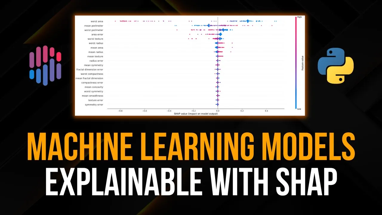









Shapley values, originally from game theory for fairly dividing game value among players, are extended to machine learning to explain how each feature contributes to a model's prediction by calculating the marginal contribution of each feature value across all possible coalitions of features, with the value function now representing the model's prediction marginalized over unused features; these values satisfy desirable properties including efficiency (summing to the prediction), symmetry (identical contributions yield identical values), null player (unused features get zero value), additivity (ensemble models combine attributions proportionally), and consistency, though exact computation is computationally expensive and requires approximation methods like Monte Carlo sampling, KernelSHAP, or TreeSHAP for practical implementation.
Shapley Values in Machine Learning: Feature Attribution
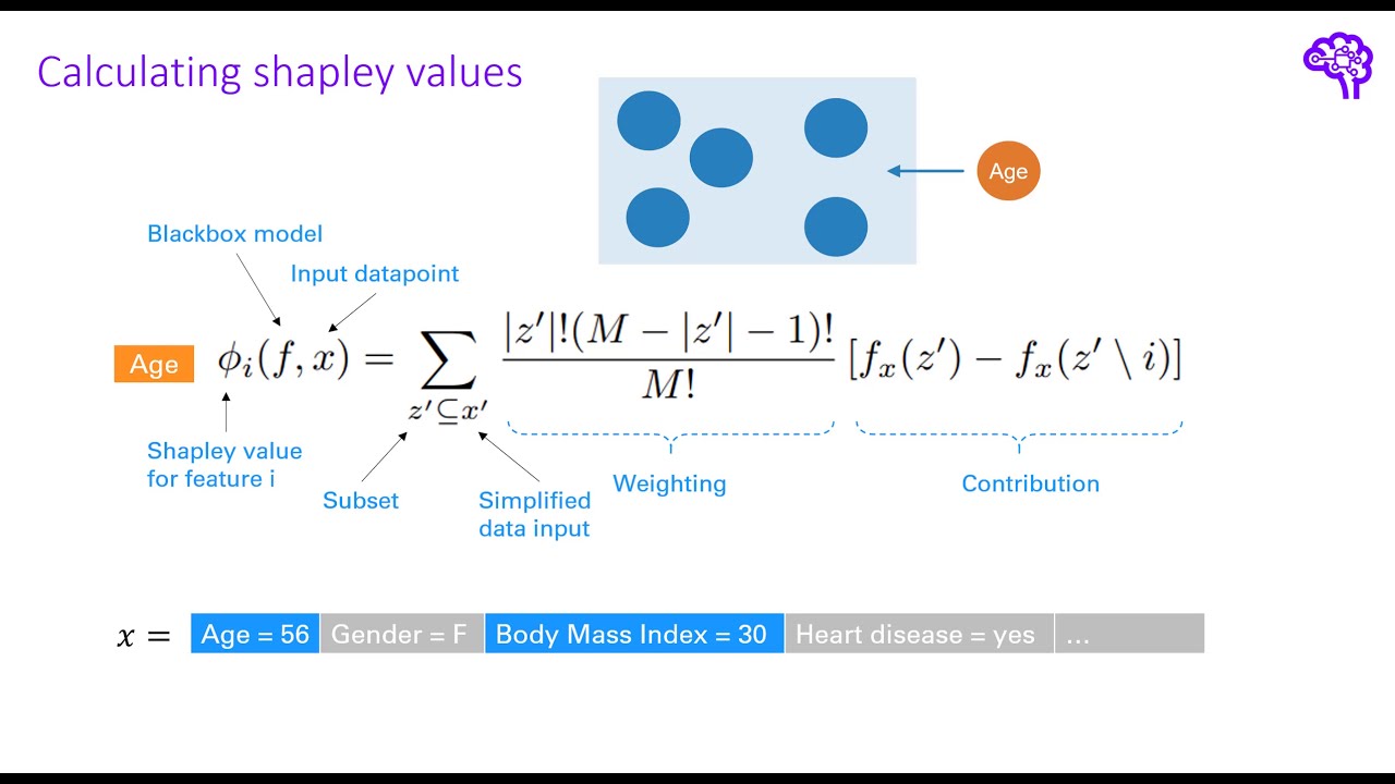
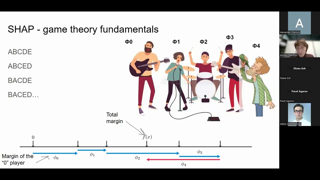
Added:sharply values come from Game Theory they were derived as a fair way to divide the value of a game amongst its players so what does this have to do with machine learning well we'll see that it's not such a big jump to go from dividing value amongst players to dividing a model's prediction amongst its features hi I'm Connor and welcome to Ado today we're going to understand how to extend the sharply value formula to explain model predictions we're also going to take some time to understand how the chappie value axioms lead to desirable properties for a feature attribution method this is one of the reasons why shop is so popular to end we'll discuss ways of approximating Sharpie values we'll see that this is the most significant reason for the package's popularity that is sharp drastically increase the speed at which we can make approximations if you want to clarify some of the details in this video then check out the companion article Linked In the description otherwise if you want to take your skills to the next level wait until the end of the video well I'll explain how you can get access to a python sharp course in a previous video we discussed this chapter value formula when applying it to machine learning we need to keep in mind that s is no longer a coalition of players but a coalition of feature values the wording can be a bit trickier you need to keep in mind that we want to explain an individual prediction all the model features will take on a value that lead to that prediction this is why we talk about a coalition of feature values but it's usually implied that we are talking about an individual prediction so often we talk about a coalition of features or the contribution of a feature to prediction or what we really mean is the features value we also need to change the value function we are no longer talking about the value of a game but the value predicted by a model so f is our model prediction and the model has P features this means the value of a coalition of features s is the model's prediction marginalized over all the features that are not in s for the features that R and S we use the actual values to be clear we are doing multiple integration to marginalize over a feature we integrate with respect to the probability of the features values we do this for all features in s to do this we need to know the features distributions or use the empirical distributions with this value function we can understand how a model has made a prediction the value of the game is now the marginalized prediction and the players are the feature values the shapley values will tell us how each feature value has contributed to the prediction so there are a lot of moving Parts in that value function to understand it let's go over an example suppose we want to predict someone's income we end up with a model f which was built using two features age which is uniformly distributed between 18 and 60 years and degree where there is an equal chance that sum all one will have a degree or not someone comes along who is 20 and has a degree plugging in these values we see that the model predicts that this person has an income of five thousand dollars we now want to calculate the sharply value for degree to start we need to calculate the marginal contribution of degree to a coalition of age we use the curly brackets to represent a coalition of features we start by calculating the value of a coalition of both features s contains both features so we do not have to marginalize over any features instead we use the actual values for both features this is the same as the prediction for this observation we then need to calculate the value of a coalition of age now s does not contain degree this means we need to marginalize over degree and use the actual value for age remember degree is not continuous to marginalize over those features values we do not need to use integration instead we sum the prediction at each value times the probability of that value which is 50 we can now calculate the marginal contribution of degree to age and this gives us parts of the calculation needed to calculate the sharply value for degree we would also need to calculate the marginal contribution of degree to a coalition of no features the other consideration is the weights for these marginal contributions and these are calculated in the same way as for a gain except now we're looking at the number of features in a coalition and the total number of features in the model Q okay that was a lot of maths and I promise it's the last okay maybe there's one more formula when we talk about the approximation methods but before that let's talk about why shop and sharply is so popular in the last lesson we spoke about the shapley axioms and in the context of machine learning these lead to some desirable properties firstly sharply values are efficient before this meant that the full value of a game is divided amongst its players for machine learning this means the prediction is divided among the features specifically the shapley values satisfies this equation the not the sum of all shapley values and the average predicted value is equal to the prediction another popular interpretation method is line and in comparison lime is not if necessarily efficient that is the weights of lime will not add up to the original model prediction for shortly we know how each feature has contributed to a prediction with lime we only know which feature is most important to that prediction the next is symmetry two features will have the same shapley values if they make the same contributions to all coalitions dummy this comes from the null player Axiom a feature will have a sharply value of zero if it never changes the prediction in other words features that are not used in a model will not have a sharply value additivity values for machine learning are additive this is only relevant for Ensemble models where the overall sharply value is the weighted average of the shapley values of all the models in The Ensemble where the weight is determined by the same weight given to the predictions of each model so for example in a random forest all of the decision trees are given an equal weight and there's actually a fifth Property called consistency this one follows from the previous three properties it tells us that if we change a model and the marginal contribution of the feature changes then the features Shakti value will change in the same direction this means we can reliably compare the Sharpie values of different models with all these desirable properties there's one thing holding sharply values back and that is calculating them is computationally expensive in our ml example we only had two features but as we add more features the number of possible coalitions increases exponentially and in practice it's only feasible to approximate shapley values one approximation method is Monte Carlo sampling how this works is we have a set of feature values and suppose we want to approximate the sharply value for feature one we randomly Shuffle the features and all the features to the right of feature one are replaced by a random sample from the respective feature distributions we get the prediction using these new feature values and subtract the prediction where feature one has also been randomly sampled this is one sample and we repeat this process n Times by randomly sampling and averaging we implicitly wait by the distribution of these features Monte Carlo sampling can still be impractical as we will need a large number of samples to get a reasonable approximation this is finally where sharp comes in the shop python package has become synonymous with sharply values and the key to the wide implementation is the speed at which this package can make approximations and it allows us to approximate a large number of shapley values and aggregate them in fact it has contributed multiple approximation methods kernel shop reframes the sharply values as parameters in a linear model the method first works by permutating feature values after enough permutations the shapley values are estimated jointly using linear regression estimating the values together is more efficient than Monte Carlo sampling where the sharply values are calculated individually Tree Shop is even faster than kernel shop it takes advantage of the structure of the individual trees in Ensemble models Tree Shop is so efficient it can be used to calculate shap interaction values the downside is it can only be used with tree based algorithms like random forests or xgboost with all these benefits shap still has its limitations these are critical if you want to avoid incorrect conclusions when using the package check out the first video if you want to understand them if you want to jump straight into applying the package and check out this second video otherwise you can get access to my python sharp cores for free by signing up to the newsletter in the description this will equip you with the knowledge and skills needed to explain any machine learning model using shop
Up Next

Explainable AI: Post Hoc Methods for Model Interpretability
@stanfordonline
16.5K views•2022-11-04

Secure Multiparty Computation (MPC): Foundations & Challenges
@SimonsInstitute
7.3K views•2015-05-28
Fairness Metrics in Machine Learning: Equal Opportunity & More
@adataodyssey
8.1K views•2023-07-30

Neural Networks Explained: Math, Layers, and Learning Fundamentals
@3blue1brown
21.9M views•2017-10-05
Related Study Plans & Knowledge Roadmaps
Structured learning paths in Artificial Intelligence