


















![(AGT4E10) [Game Theory] Shapley Value](https://i.ytimg.com/vi/HWRHKs3O_Us/maxresdefault.jpg)


SHAP (SHapley Additive exPlanations) is a Python library that explains machine learning model decisions using Game Theory principles, allowing users to visualize feature importance through summary plots and understand individual prediction decisions through force plots, even for non-inherently explainable models like Support Vector Machines.
Machine Learning Model Explainability with SHAP in Python
Added:Proficiency in Python programming and core data science libraries such as Pandas, NumPy, and Scikit-Learn.
Fundamental understanding of supervised machine learning concepts, specifically how classification and regression models are trained and evaluated.
Familiarity with 'black-box' ensemble models like Random Forests or Gradient Boosting (e.g., XGBoost, LightGBM), which are primary targets for interpretability tools.
Comparing and integrating SHAP with other Model Interpretability frameworks, such as LIME (Local Interpretable Model-agnostic Explanations).
Applying SHAP values to detect and mitigate algorithmic bias, ensuring fairness and ethical compliance in machine learning decision-making.
Deploying Explainable AI (XAI) in production environments, including building interactive explanation dashboards (e.g., using Streamlit or Dash) for stakeholders.
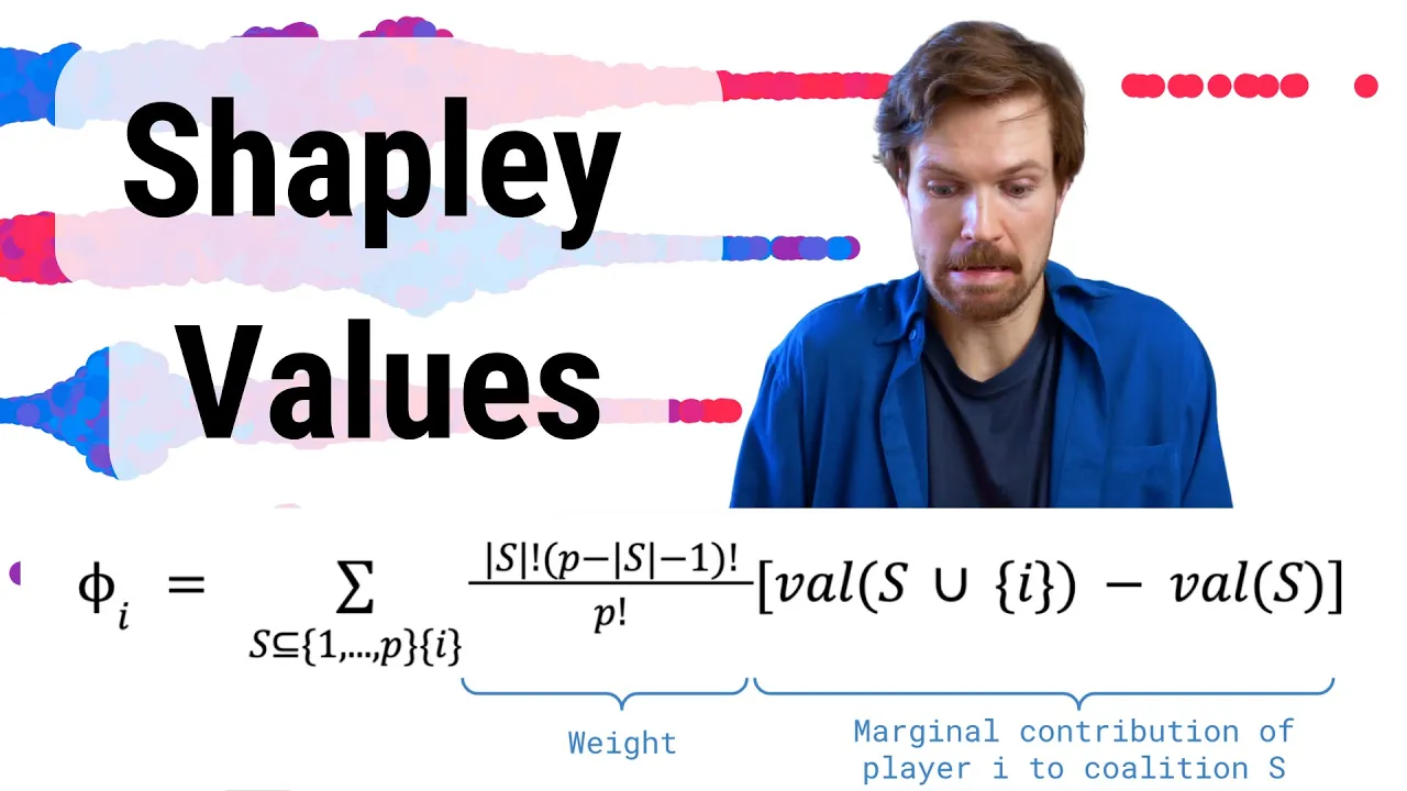
Deepening theoretical understanding of Cooperative Game Theory and the exact mathematical formulation of Shapley values.
10.1K views343likes13:31Original Release: 2024-02-26
what is going on guys welcome back in this video today we're going to learn how to explain the decisions of machine learning models using shap or shap Le in Python so let us get right into [Music] it all right so we're going to learn how to explain the decisions of machine learning models using shap in this video today and shap stands for shly additive explanations you can see this is not necessarily the most intuitive way to come up with the acronym but this is what it stands for and it's based on Game Theory now I'm not going to focus too much on the theory in this video today or actually I'm not going to focus on the theory at all if you are interested in understanding how shap Works behind the scenes let me know in the comment section down below if enough people request it I will make a video on it uh but other than that I'm going to focus today on the Practical part and on the application of shap in Python I also recently made a video about lime which stands for local interpretable model agnostic explanations uh which is also a way of explaining machine learn machine learning models that are not inherently explainable uh and today we're going to learn about shap which works differently now some models like decision trees for example are inherently explainable they have a literal decision tree that you can look at and it explains exactly how a conclusion is reached so you get some data and then you classify it as zero or one as uh good or bad is black or white or as in this video today malignant or benign we're going to look at tumors um and the decision treat tells you exactly what the model does to get to the conclusion it looks at certain values at certain thresholds and it says yes no uh higher or less than greater than or uh lower than some value and then it comes to a conclusion this is good or bad malignant B9 whatever and some models don't do that some models just give you the prediction so for example support Vector classifiers they will give you a zero or a one they will not even give you probabilities they will not give you feature importances and they will definitely not explain the decision Mak process they cannot explain the decisions the individual decisions that they make and in cases like this things like lime or shap are very useful so what we're going to do first now is we're going to open up a terminal and we're going to install a couple of packages first of all of course the shap package which is for shap itself then we're going to also need numpy probably also mat BL lip I'm not sure um and we're also going to need pyit learn for the machine learning part and then we can start by importing shap by importing numpy S&P and then from sklearn we're going to import the data set so from sklearn data sets we're going to import load breast cancer which is a function that will give us the data set then we also want to have from SK learn model selection the train test split function so that we can split our data into a training set and a testing set and then from sklearn.svm support Vector machine we're going to import the linear support Vector classifier which is not giving us any explanations out of the box so what we're going to do now is we're going to say X and Y is equal to data data and data Target then you can look at X it's basically just the parameters and Y is0 or 1 so malignant is 0o 1 is been n you can see that this is the case by just printing the target names so data Target names like this you can see Zero is malignant one is benign and uh now what we're going to do is we're going to split this into XT Trin X test y train y test this is going to be a train test split from X and Y with a test size of 0.2 So 20% of the data will end up in the test set so what we're going to do now very easily usually when you do a linear support Vector classifier when you train a linear support Vector classifier you want to scale the data it's not too important now we're just going to uh say classifier is equal to linear SVC and then we're going to say classifier fit on XT train and on y train and we can actually then also say clf do um score and we can score it on the X test and the Y test data you can see we get 92.9% accuracy probably this is going to increase I assume if we scale it before but it's good enough to to uh for for the purposes of this video today so what we want to do now is we want to understand how does the linear support Vector classifier make a decision because if I go ahead and I say cf.
predict I can of course pass an instance for example the first instance of the test set and I'm going to get a prediction one but it doesn't tell me how it gets there it doesn't explain to me what exactly is happening uh for this to be classified as uh benign in this case as one so what I can do now is I can do the following I can say explainer is equal to sh. Kernel explainer and what I pass here is first of all the predict function so cf. predict and I also pass a sample of the data so I can say shap do sample or sh. k means we're going to do K means in this case uh K means basically summarizes the data uh with centroids and Sample just samples from the data so what we're going to do now is we're going to pass from the train data we're going to pass the train data and we're going to pass 10 to the K means function um and then we're going to get the actual shap values again not going to explain how exactly this happens now behind the scene but we get the shap values from the explainer by doing explainer do shap values and we're going to pass the test set here now this is going to be calculated as you can see this takes some time and of of course the larger your data set and the more complex your data set the more time this is going to take but then we can very easily just produce a summary plot and the summary plot doesn't even focus on a single instance it focuses on the classifier in general so what we can do now once this is done we can say shap do summary plot and we pass the shap values we pass the test data set we pass the feature names which are going to uh going to be data feature names and um then let me just see if we need some more parameters no I think that's it then what we get is this here and basically the idea is the following here you can see on the xaxis we get the impact on the model output meaning if it's close to zero it's not that relevant if it's very much to the left or the right it's relevant so depending on the direction of course what you can see basically here also the color indicates whether the value is is high or low and basically um this means that the worst area being high is an indication for this being classified as zero whereas the worst area being very low is pushing the model towards classifying it as benign um and it's the other way around here so very low values indicate um malignant and very high values indicate benign so that is a summary plot of the whole thing already here you can see how the features impact the model but we can also go a step further uh we can explain individual decisions so what we do for this is we say sh. init JS this is just necessary here in a notebook to display uh the plot and then we can display a so-called Force plot seeing how the individual features apply forces uh to to uh basically come to a decision so we can say explainer do expected value then we're going to say shap values Zer because we're classifying just one instance here X test zero and then again we get the feature names is equal to data feature names and what you can see here now now you cannot see all of this because unfortunately uh it doesn't it doesn't adjust this with a dark mode but maybe you can see it in the video if not just believe me it's there uh you have some text here that is black on dark gray so maybe you cannot see that but it says here basically a couple of values and then it says here importantly base value and base value is 0.673 this is the uh base value and then you can see the individual features push the prediction towards something so the worst area being this value here pushes the prediction very far to the right uh towards a classification of one towards a classification of benign and then this being that value also pushes it then some small pushes here some large pushes also against um the classification of one pushing it more towards malignant but in this case you can see here um that the left side is much larger so this is how you can explain individual decisions I can also change this now uh to another instance or to get another instance maybe we can get a zero somewhere no seems like we only get to Once let's do one more if it doesn't reduces zero okay doesn't matter but you can see here now how you can explain individual decisions being made on individual instances now with all this we can also generate uh some sort of feature importance so what we can do here is we can say import or actually I have numpy imported already right yeah uh we can use numpy to take all the shap values to summarize them to aggregate them basically and to take the absolute value of them so that we don't really care about how it influences the model just that it influences the model and we can do that by saying mean absolute shap values is going to be equal to NP absolute shap values and then we take from this the mean on axis zero this will give us the mean shap values and then we can take this and turn this into uh we can display this as feature importances so we can say feature names is equal to data feature names then we can say uh feature importance is zipping together the feature names and the mean absolute chap values um and then we already should see okay actually we would have to turn this into a dictionary to see um the feature importances but now we can also sort them so what we can do is we can say um sorted feature importances is equal to sorted feature importance and the key is equal to Lambda X and we sort by X1 reverse being equal to true because we want to have from highest to lowest uh and then actually we can just what does it look like right now sort it come on where just the auto complete uh this does not look like it worked did it not true about this oh there you go um and now what we can do is we can basically just iterate over it so we can say say for feature and [Music] importance in sorted feature importances print and then just feature importance and you can of course uh turn this into maybe we want to have a colon in between like this but that is basically now our feature important so this is um how important the individual features are the most important one being the worst area mean perimeter and so on and this is all on a linear support Vector classifier that doesn't provide probabilities doesn't provide feature importances and doesn't provide any explanations of how it gets to the conclusion you can explain models like this but also of course uh random forest classifiers and uh basically all the different kinds of models you can explain with shapley like this or with shap like this uh yeah this is a very nice thing and a very nice uh alternative to line so that's it for today's video I hope you enjoyed it and hope you learned something if so let me know by hitting the like button and leaving a comment in the comment section down below and of course don't forget to subscribe to this Channel and hit the notification Bell to not miss a single future video for free other than that thank you much for watching see you in the next video and bye
Up Next
6:47
Writing a x86 Bootloader in Assembly with NASM
@nirlichtman
50.3K views•2023-06-10

87:26
Introduction to Secure Multiparty Computation with Yehuda Lindell
@fhe_org
7.7K views•2021-02-04

38:48
NetworkX for Graph Theory: A Python Crash Course
@NeuralNine
104.6K views•2023-02-01

19:25
Enigma Machine Mechanics: WWII Encryption Explained
@JaredOwen
13.2M views•2021-12-11
Related Study Plans & Knowledge Roadmaps
Structured learning paths in Computer Science
computer-science
Container Runtimes: Namespaces, Cgroups & Go
01Linux Systems & Go Programming Foundations
02The Core of Isolation: Chroot and Filesystems
03Linux Namespaces: Process Isolation
+ 3 more learning modules
32h6 modules
Explore Roadmap
computer-science
Building a CHIP-8 Emulator: Rust & CPU Basics
01Computer Architecture Foundations (Bits & Bytes)
02Rust Programming for Systems Development
03CHIP-8 Virtual Hardware Specifications
+ 2 more learning modules
32h5 modules
Explore Roadmap
computer-science
Building BitTorrent: Go, P2P & Concurrency
01Go Fundamentals & Concurrency
02Networking Foundations & P2P Architecture
03Bencode Parsing & Torrent Metadata
+ 3 more learning modules
26h6 modules
Explore Roadmap
computer-science
Actor Models (C++ Concurrency & Lock-Free)
01C++ Multi-Threading Foundations
02Thread Pools and Task Scheduling
03Atomics and Lock-Free Queue Design
+ 3 more learning modules
45h6 modules
Explore Roadmap