














This lecture covers the fundamental concepts of evaluating machine learning algorithms, including error measurement (absolute error, sum of squares error, and misclassification rate), the confusion matrix framework for classification (with TP, TN, FP, FN), and key evaluation metrics like accuracy, precision, and recall. It explains the critical distinction between sample error (measured on training data) and true error (actual performance on unseen data), identifying four main sources of error: representation bias, search bias, variance error, and noise. The lecture introduces the standard validation procedure with training, validation, and test sets, and presents K-fold cross-validation as a method to maximize data utilization while obtaining reliable error estimates when training data is limited.
Evaluation and Cross-Validation in Machine Learning
Added:Good morning.
Now, we will start Part d of Module 1.
In this module, we will talk about how to evaluate learning algorithms.
We will do a preliminary lecture on evaluation and how to use cross validation for the evaluation.
This will be the topic of the current lecture.
So, when you have a learning algorithm you have to and just find out.
As we saw in the last module that given a hypotheses space H, given a training data S your learning algorithm comes up with h belonging to capital H. Now, it is important to understand how good h is right.
So, you want to do evaluate the performance of learning algorithm and you can come up with experimental evaluation.
So, you must have a metric by which you evaluate.
So, different matrix can be used, for example, you can have some sort of error metric, you can find out what is the error made if you assume h as the function.
You can look at accuracy, you can look at precision recall and some of these things we will define now and in order to evaluate the error you can evaluate you can find out the error, accuracy, precision, recall etcetera on a sample.
So, you can evaluate the error or other parameters on the training set, but since you are using the training set to come up with the hypotheses the error or accuracy that you get on the training set is not, may not be a reflection of the true error, because of that you use a test set which is disjoint from the training set and we will talk about cross validation, which can be used while training the algorithm in order to tune the algorithm.
How you can split the training set into train and test and still use the data that you have to your maximum advantage that can be discussed when we discuss cross validation.
Now, how to evaluate a prediction?
Suppose you have come up with h and you get an example x and you want to make a prediction on x.
So, you want to make a prediction on x, h (x) and let us say h (x) equal to y or we can say y hat equal to h (x) and suppose associated with x the correct value of y is given.
So, y hat is what you have predicted and y is the actual value of y.
Now, if y hat and y are same then there is no error and if they are different there is an error.
So, if y hat differs from y there is an error and we have to discuss how this error is measured.
There are different ways in which error is measured.
We will talk about some of them absolute error is measured by h (x) minus y.
So, h (x) is your y hat.
So, h (x) minus y is the absolute error on a single training example.
If you have n training examples this is the absolute error on a single training example.
If you have multiple training examples, let us say n training example then you can take the average of that.
Then you can have sum of squares error.
In sum of squares error, you look at h (x) minus y whole square and then you take summation and average of it.
So, this is sum of squares error.
So, absolute error and sum of squares errors are especially useful for regression problems.
For classification problem, you can look at the number of misclassifications, which can be defined to be 1 by n sigma i equal to 1 to n delta h (x), y.
So, delta is a function which returns 1, if h (x) and y are different and 0, if they are same right.
So, this is the number of misclassifications divided by the number of examples on which you have tested.
These are some differ measures of h.
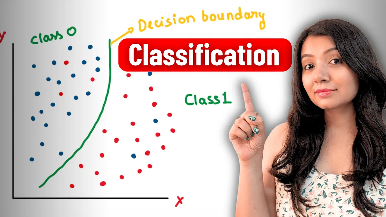
Sometimes, especially in classification problem it is helpful to define a confusion matrix.
In a confusion matrix, you can denote; suppose you have a two class classification problem and you have a set of examples on which you are testing and on this side you have the true class and on this side you have the hypothesized class.
So, the true class can be positive or negative and hypothesized class can be positive or negative and those training examples for which the true class is positive and you also hypothesize positive they can be called TP.
The numbers of such examples are put in this box.
Similarly, TN stands for true negative, those examples where the true negative classes are also output as negative by your learning algorithm will come here.
So, these are the zones where your learning algorithm predicts correctly, but your learning algorithm can also make mistakes and there are two types of mistakes; false positive means the examples are actually negative your learning algorithm is wrongly classifying them as positive, and false negative means the learning algorithm erroneously marks as negative, those examples which should have been positive.
So, this is a confusion matrix and you can have a confusion matrix if you have more than two classes also, for example, if you have three classes as an output to a classification problem you will have 3 by 3 confusion matrix and the diagonals diagonal entries are the ones, where the learning algorithm is giving the correct result and the non-diagonal entries are where the learning algorithm is giving the wrong result.
Now, given this entries in the confusion matrix accuracy can be defined to be.
So, TP and TN are the correct results.
So, accuracy is TP plus TN divide by all the examples.
So, let us say that sum of this column is P; sum of this column is N.
So, we can say it is a TP plus TN by P plus N. Along with accuracy, we are sometimes interested in other measures, for example, precision is defined to be out of the examples that the learning algorithm marks as positive, how many are correctly positive?
So, precision is defined to be TP divided by TP plus FP.
So, TP plus FP is what this row is what the learning algorithm defines to be positive, out of it TP are the ones which are actually positive.
So, this defines precision and we have another measure called recall which measures how many of the positive examples the learning algorithm retrieves as positive.
So, recall is taken to be TP by P and P is TP plus FN and this is also called true positive for 8.
Similarly, you can have a false positive for 8.
These are some ways in which we can evaluate learning algorithms.
Now, the next thing we will briefly discuss is on what data we evaluate the learning algorithm.
So, we are evaluating the learning algorithm on a sample data and the measure of error, suppose we are trying to measure error the error that we get on the sample is called sample error, and the actual error is called the true error.
So, let us look at a classification problem.
The sample error of a hypotheses f with respect to a target function c, and data sample S is the average number of misclassifications.
So, delta f (x), c (x) sigma of delta f (x), c (x) is the number of examples, where f (x) and c (x) do not agree.
This is the number of misclassifications divided by n, this is the sample error.
Now, the true error is defined over the distribution of instances, right there is a population of instances from which we assume that the samples are drawn and the true error is with respect to this distribution.
So, the true error of a function f is the probability that on this distribution f (x) and c (x) will not agree, this is the true error.
So, we have the sample error which we measure with respect to a sample and there is a true error.
Now, what we really want is the true error and when we take the sample error there is some error.
Now, when you hypothesize a particular function the error that you get comes from different sources.
The error can come from the limitation in the representation function or the limitation in the hypotheses space and we have discussed that this is due to bias in representation.
The error may come because given the hypotheses space the search algorithm is not exhaustively searching the hypotheses space, but making certain simplification that is called search bias.
The error may be due to the limited size of the sample that you use for testing then it is called variance error and error could be because the features that you are using the vocabulary that you are using is not sufficient to capture everything about the task then this is called a this is called noise.
So, there are different sources of error in a learning algorithm you take a sample and you find the sample error and the sample error may be different from the true error.
So, we have to understand what type of errors can there be.
Now, when you make this estimate from the sample as we saw that there could be error due to bias in the estimate and the sample error may be a poor estimator of the test error, and if you choose the sample to be the training data then you are making a very bad decision about the true error because the hypotheses you have learned from the training examples only.
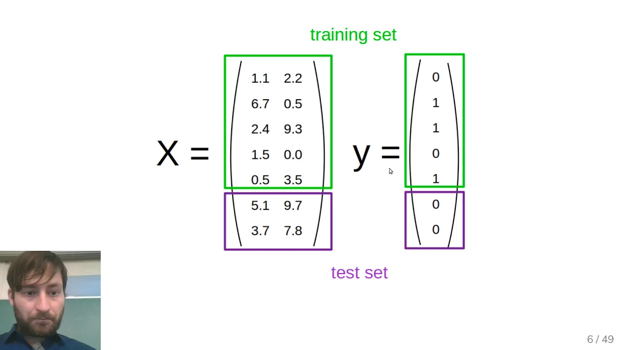
So, what you need to do is you split the examples.
You use some examples for training and you use a disjoint set of examples for testing, and ideally both the training set and the test set are drawn from the distribution.
So, the training set or the training examples are use to train the learner and the test set is used to test the learner.
So, this is about bias.
There could be also be variance in the estimate as we said if the test set is small there will be variance.
If you take a small test set coincidentally the accuracy may be very high or very low on that set.
So, if you take a larger test set the variance will be smaller.
Now, we will look at a way of doing the evaluation with limited training data.
So, suppose if you are given some labeled data, right.
Now, if you use up all the data for training you will not be able to really get a good estimate of the error because you require an independent set.
So, what you should ideally do is given the examples you will divide the example into training set and test set, but when you do this division the size of the training set will decrease and we will see that if the size of the training set is too small it will give rise to over fitting type of error.
So, you want to use as much of the training example as possible for training and also we do not want to test on a small test set if we test on a small test set variance will be high.
So, you want to use all the examples for testing for that we evolve a scheme for cross validation.
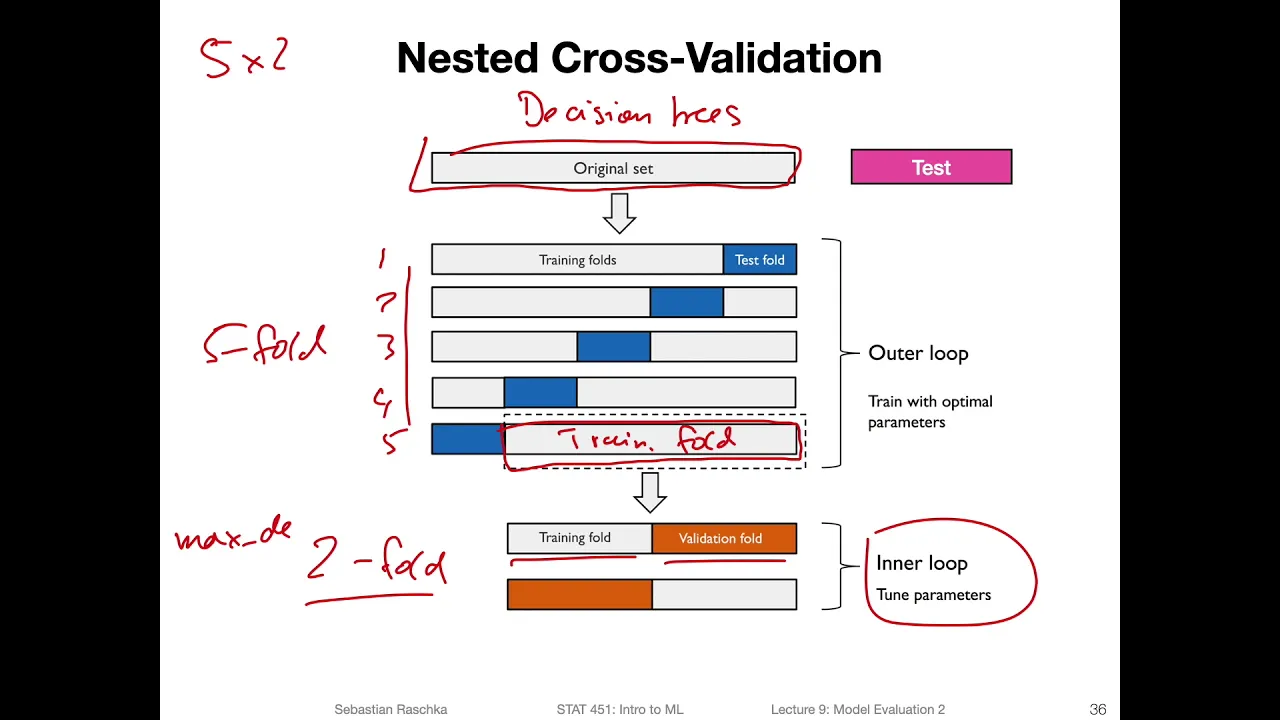
So, if you look at this slide given the original set of examples, we can first split the data into training set and testing set.
So, that the testing set is completely disjoint for training.
During training when you are tuning the model parameters you can use some part of the training set for validation.
So, for the training you use training and validation and after you have finished tuning, the whole thing whole the hypotheses that you output is checked on the testing set.
This is the standard validation procedure.
So, validation set is used during tuning during training to tune the model parameters.
After the entire training is over then you check your answer check the accuracy of your hypotheses on the test set.
So, when you do validation if you are splitting your data into these parts validation fails to use all the available data.
So, we will come up with a scheme called cross validation.
Let us look at what is K-fold cross validation.
In K-fold cross validation, what we do is that we take the entire training data that is available to us and we split it into K classes.
So, suppose K equal to 6, we will split the data into K subsets right then we will perform K experiments.
So, K rounds of learning.
In round i we will use; suppose this is S 1, S 2, S 3, S 4, S 5, S 6.
In round i, we will use S i for testing and S minus S i for training, together this is S. So, at every round, 1 by K of the data is set apart for testing and the remaining examples are used for the training.
So, we will have K experiments and after this K experiments are over the test score that we will output is average of the error of this K rounds.
So, we are using the different parts of the data for testing in the different rounds.
So, this is called K-fold cross validation.
This is illustrated by this picture here; this is round 1, round 2, round 3, round 10.
There are 10 splits of the data in this picture and in round 1; suppose the accuracy is 93 percent, round 2; 90 percent, round 3, 91 percent and so on till round 10; 95 percent and the final accuracy is the average of the accuracies in all the rounds.
This is called K-fold cross validation which makes use of limited data, so that the training and testing can be done at all points.
Now, in machine learning as we will see now and subsequently there is always a trade-off, there is a trade-off between complex hypotheses, complex representations and simpler hypotheses.
Complex hypotheses can fit the training data well, they are more flexible, but they have a tendency to over fit the training data and may work poorly on the test data especially if the size of the training data is small.
On the other hand simpler hypotheses may generalize better, but they may not be able to represent complex functions, if your training data is large then the generalization error will decrease and you can go for complex hypotheses.
With this, we come to the end of the introduction module and with this brief introduction and the different issues that we have touched upon.
In the next module, we will start with the description of some of the learning outputs.
Thank you very much.
Up Next

Stanford CS229: Bias-Variance Tradeoff, Cross-Validation & Regularization | Lecture 12
@stanfordonline
20.6K views•2021-04-20

Secure Multiparty Computation (MPC): Foundations & Challenges
@SimonsInstitute
7.3K views•2015-05-28

Bypassing Tor Censorship: Bridges and Pluggable Transport Guide
@Coding_ForEveryone
397 views•2024-06-11

Neural Networks Explained: Math, Layers, and Learning Fundamentals
@3blue1brown
21.9M views•2017-10-05
Related Study Plans & Knowledge Roadmaps
Structured learning paths in Artificial Intelligence