












![Linear Regression - Intro, Assumptions & Code [2021-02-22]](https://i.ytimg.com/vi/zogCJCYHGac/maxresdefault.jpg)
![로지스틱회귀 wih MATLAB / 인공지능 프로세서 실습 20-6[실시간 원격 수업]](https://i.ytimg.com/vi/P3csuOuQaaY/maxresdefault.jpg)



![HIMTI Responsi 2026/2027 | Machine Learning [B28] | UTS Semester Genap](https://i.ytimg.com/vi/3tgRb2nPJJw/maxresdefault.jpg)







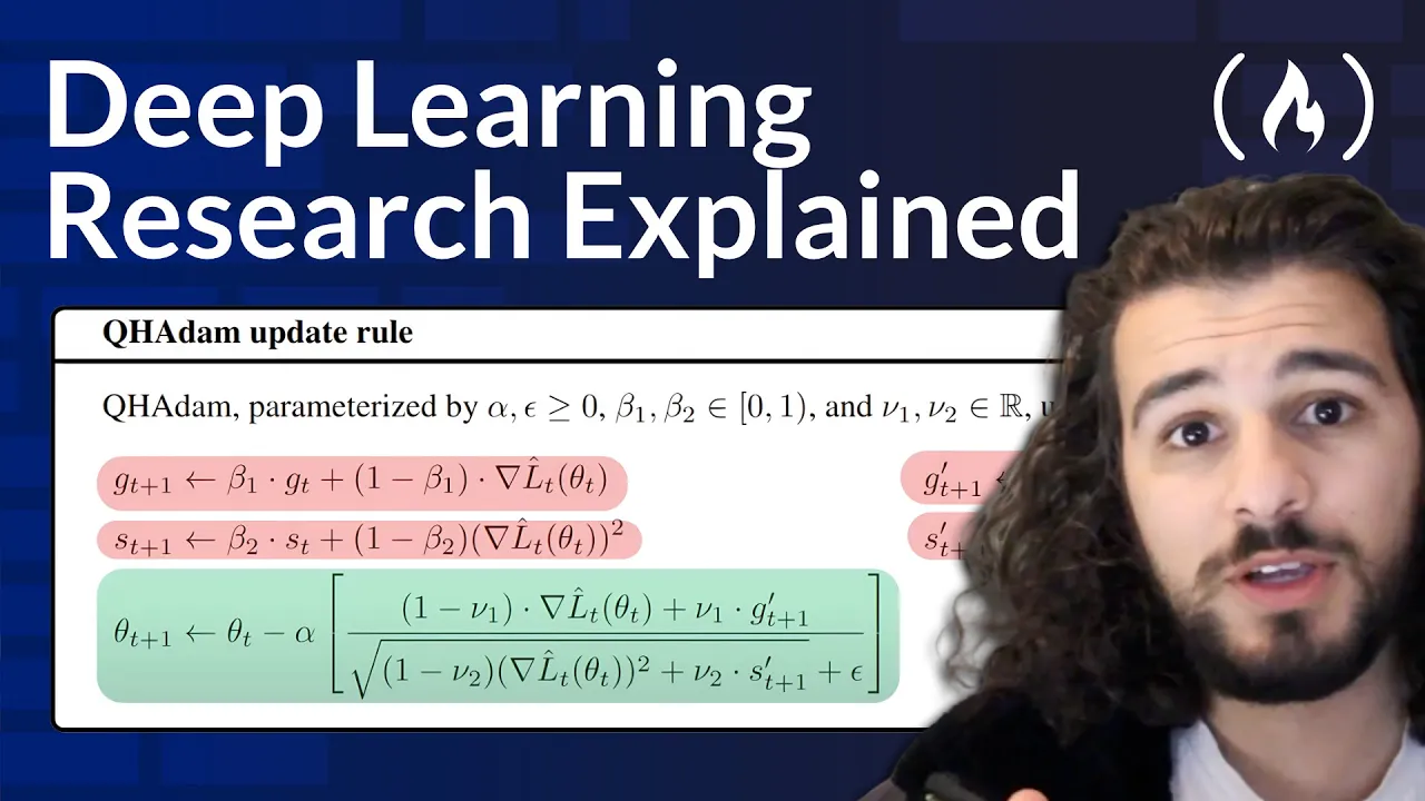
Linear regression is a statistical method that uses a straight line equation (y = mx + c) to model the relationship between an independent variable (X) and a dependent variable (Y), where m is the gradient and c is the constant. The training process involves minimizing the cost function (typically Mean Squared Error) through gradient descent, an iterative optimization algorithm that adjusts parameters by moving in the opposite direction of the gradient, scaled by a learning rate. The algorithm continues until it converges to the minimum error point, where the cost function no longer decreases.
Linear Regression with Gradient Descent | KodeCamp 5X ML Class 4
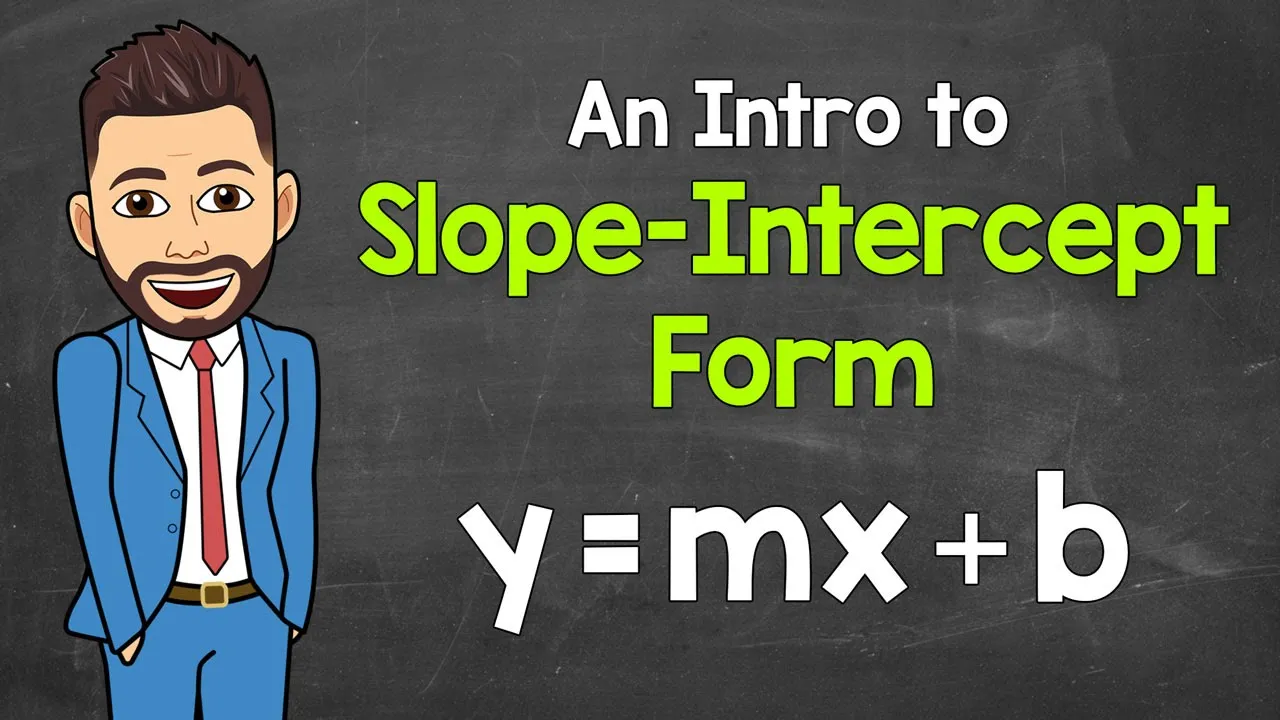
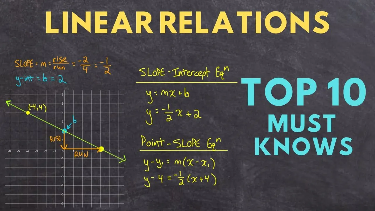
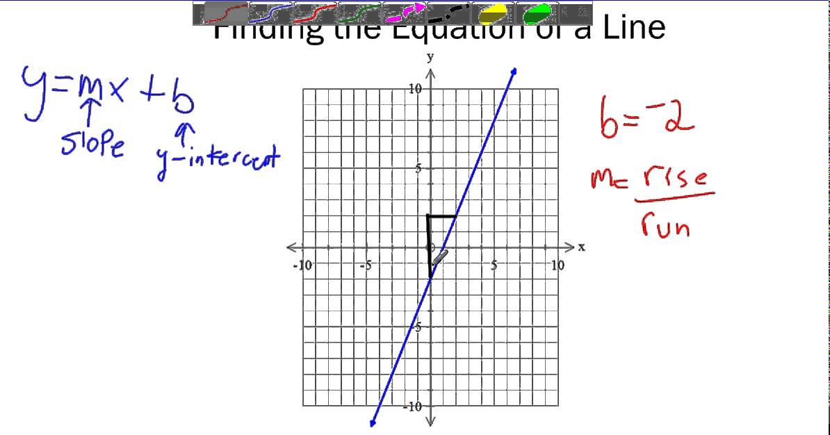
Added:Basic algebra, specifically understanding the equation of a straight line (y = mx + b), slopes, and intercepts.
Introductory calculus concepts, particularly how derivatives represent the rate of change and how they are used to find the minimum of a function.
Basic statistical concepts, including independent and dependent variables, data variance, and the general concept of fitting a model to data.
Fundamental programming skills in Python, including working with variables, loops, functions, and basic library structures like NumPy arrays.
Multiple Linear Regression, to understand how to scale the model to handle multiple input features instead of just a single predictor variable.
Regularization techniques such as Ridge (L2) and Lasso (L1) regression to control model complexity and prevent overfitting.
Logistic Regression, which transitions the concept of gradient descent and cost functions from continuous prediction to categorical classification tasks.
Advanced optimization algorithms, including Stochastic Gradient Descent (SGD), Mini-batch Gradient Descent, and momentum-based optimizers like Adam.
400 views10likes1:51:35Original Release: 2025-11-07
Okay, good evening once again everyone.
So today we are going to take a look at more of linear regression. Last Monday we had started off uh talking about linear regression. We spoke about uh the process of training a model and we spoke about uh data pro processing pre-processing and then we looked at the five stages of training data input forward propagation loss calculation backward propagation and parameter optimization today. Then of course we did a bit of linear regression with single variable. So in this case I was manually adjusting the parameters. So you remember we tried to um simulate or predict the values of a system of um um data points. You know the values of data points based on a linear equation which is really what linear regression is is a statistical method. We use a straight line to model the relationship between a single independent variable which we call X and the ind and the dependent variable which we call Y whose value comes from the value of X. And then the specific value of y depends not only on the value of x which is the independent variable but it also depends on the parameters around x which include m that we call the gradient or the coefficient of x and c which is also another coefficient but it is a constant. So by adjusting the values of m and c which is what we actually call the training process in machine learning. In this very simplistic example, we are able to adjust what the model will predict as the y depending on what value comes in as x. So in this case, the model is actually this single linear equation y = mx + c. That is the model and nothing more than that. So when you hear a machine learning model, it's basically a system of linear equations like I have said and um each of the coefficients in this lead linear equation or this system of linear equation is what we call the parameter and those are and lots of them will make up all of the parameters. Of course, what you'll be asking yourself now is how can you know this number of uh you know a large number how do do these parameters even come together to make sense and learn a complex thing like you know AI you know composing a poem or a letter or you know doing some playing chess you know all of that so that's part of this interesting journey of machine learning how do we move from this single linear equation y= mx + c to charg it is an interesting um you know question and we're going to see that so with linear regression you are basically using a single straight line that's why it's called linear to predict your models the model in this case is the equation this the straight line equation that's the model so you use that to predict a value Right? So the best way to do that is you look for a straight line that is going to minimize the error you know of prediction versus the actual value. So for you to do that you have to first of all create what we call a loss function or a cost function.
those are um the you know terminology that is used. So the cost function will calculate the difference between the predicted value and the uh actual value.
So what we call the error.
So that error there are different types of loss functions right or cost functions. Um in both cases they mean the same thing. So you have a mean squared error as an example, right?
That's one. And I explained how that works. It's basically the average of the sum of the squares of the error or the difference between predicted and actual for each data point. So that is what this function is.
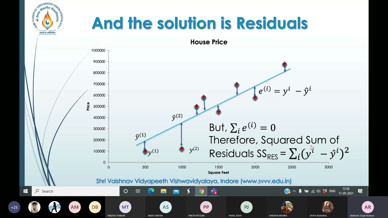
Basically it's a summation across all data points. The all data points are from i being 1 to i being n. So i is the i here y i right minus mx i + c. So remember mx + c is yhat. If you look at the previous one, yhat is a terminology we use for the prediction that comes out from the model. So you calculate that difference for each data point. That's why you have the I the I represents a single data point. So for n data points which is the total sample of data points that are given to you as part of the training data you square right then when you square you sum sum it that's what this summation symbol stands for and then you divide it by n which is again the total number. So when you divide a sum by the total number of um of samples right or of items in that sample or data points in that sample what you get is an average or a mean. So that's why this is called a mean squared error. You also have m ae which is the mean absolute error. So the mean absolute error instead of squaring inside this summation you take the absolute value which the absolute value is basically ignore the sign whe whether it's positive or negative forget the sign just take the value which is the number which obviously means you only take the the positive value and you sum it up so the essence of using squares like I said before or using absolute is we don't want negative and positive errors to cancel each other out because we are not trying to calculate the sum of the errors. We are trying to calculate the magnitude of the total error in the system. So you have to remove the sign so that they don't cancel each other out. So when you do that you get this equation. Now your goal is you want to train this model so that you minimize this total error as measured by the mean square error or any other um cost function that you choose.
So to minimize this right, you will now um adjust the parameters in the model in this case the M and the C. And if you were to plot a graph as you adjusting the M and the C, which in this case are the weights, you would see that the error drops at up to a certain point. A certain point hits a minimum value. But if you continue adjusting it, the error begins to increase back. So what that means is that there is a point of minimum error. That is the goal. Your goal is you want to get to that point of minimum error. So what is the next step?
There are two ways to solve this kind of linear regression. The first one is the analytical method where to find this minimum point you use the simple mathematics that we have learned. Right?
Which is the point of inflection or the minimum point is a point where the change in the cost function or this gradient is zero. The gradient of the cost function itself. Not the gradient of the predicted value or not the gradient of the model of the of the line that you are using to predict. No, not that one. But the gradient of this cost function right at the point where it is zero that is represented by d delta j delta m or del j del m you get zero that is the gradient. So the only thing is that we use a partial differential approach because it has been proven that you only need to adjust each parameter to a point where its own contribution it's the minimum. So if each parameter you adjust to a point where each parameter's own contribution to the error is a minimum, you would have successfully minimized the entire error in the system. So you you don't need to consider the um we assume that these parameters are independent. They they don't they're not coupled in any way mathematically or otherwise. So we can adjust m to a point where the change in the cost function with respect to m is zero and we do that math. We can also adjust j to a point where the the change in the cost function which is del j with respect to the constant c which is second parameter is also zero. So this curve applies to both the m and the c.
So you can actually see that even though it's written weight here but this same curve applies to the JDM to M right as you're adjusting M it gets to a point where the cost function which is on the Y ais becomes uh at the minimum and at that minimum point the rate of change of that cost function with respect to the m parameter is zero. Same thing we see. So this curve applies to both. Now what do you do? The next thing is you take this formula and you do the necessary maths with it. Right? Unfortunately, I do not have enough time to go into the math of this and I'm not really going to go into it because that's not really the purpose of our training. Our training is not for you to learn regression using analytical methods, which is what this is, right?
but rather using numerical methods which is um iterative adjustment right and that is um for example what a gradient descent will do for you so I'm not going to go into the maths it but just take it that by the time you take you take the the derivative of the cost function right and set its value to zero and reverse calculate the m you are going to get this formula. You make m the subject of the formula you're going to get m you're going to get this formula for m right you can actually see that here right if you do a derivative of this and I'm going to show you this in another slide but if you do a derivative of this is going to give you 2 yi minus um mx + c in brackets, right? Times x, which is going to be 2x i y i - 2x i into y i - mx + c. So that will give you an equation which when you make m the subject of that formula you're going to get m as n * summation of x i y i minus summation of x i * summation of y i over n * summation of x i 2 minus summation of x i all^ 2. So um again it would have been interesting for me to delve into this but I'm going to spend a lot of time and today is jam-packed but just understand you can go do it as an exercise on your own right that by the time you take this first equation where we say del J del m equals to zero you do the derivative the partial derivative this dell by the way we call it dell is is just short for delta I could have said dj DM but the JDM is um where you don't where you have a single variable so it's a derivative but when you have partial derivatives we typically use this other d instead of a straight d we use this so this formula by the time you um do that derivative like I said make it subject formula you get this for m so you can now slot in all the values of x and y and do this calculation and you will solve for M this is a one what we call um a one touch right or a one shot. It is a one shot right. So the one shot is it means you calculate the correct M the minimal M at a single go right. So that's one benefit of using an analytical method.
You just do a single calculation. You don't need to do iteration. Right? But you also see where the iteration is more powerful than this. We'll talk about that. So similarly if you also take this second differential equation where you are calculating the uh contribution of the C constant to the cost function which is del J del C and you you take the derivative of this J with respect to C. You are going to get 2 into Yi minus U MX I minus C. Right? That's all you get. So you can then flip it and make C the subject of the equation and you get this back that C equals summation of Y I - M summation of X I / N. So this gives you a single equation for you today oneshot calculation of the C right which is the second parameter that is linear regression using mathematical sorry analytical methods like the mathematical equation that we were used to. Now this works well if you already know the cost function right so I can actually do this and it's really nice I can do this right you can even use this and program it in a computer because you already know the equation to use you know you are using a cost function of um you know mean square error because the mean square error that is going to give you this um derivative when you flip the formula Right? But if you use a different one, it will be a different thing. So in this situation here, we use that same analytical method to just uh slotting the values into that those equations that we had. And we immediately calculated that C for these three points X and Y points. C is 1.214.
Sorry, M is 1.214 and C is 0.19. And you can slot that to get your equation. Y = 1.214X. 214x + 0.19. This is the model.
In fact, you can consider this as a trained model. It has two parameters.
1.214 which is the M and 0.19 which is the C. And this is the um values of this. This is the values of the two parameters that will give you the list error. So you can say with this I can do a a good prediction.
I am using this very simple case to explain so that when you are visualizing in your mind what is a model, what does parameter mean, what does even look like you know like people have been asking you know that these are just floating point numbers like I said that have been adjusted by training. Now here it is we just solved it one shot and we got the answer. But the there is a downside for really complex systems. You cannot come up with an equation that does that or if you were to come up with such an equation, it would take too long to calculate even with the fast computers we have today. So we come up with a second approach which we are going to talk about. By the way, this is a visualization of the results. So you this is a good example where well this is not actually exactly this data point but um this is it now yeah I did a hands-on session where I tried to explain how we could do this right using um you know a manual process of adjusting the parameters but I'm not going to do that rather what I'm going to show you is a a Jupyter notebook I had already done right which kind of does that linear regression. So you can see all of this it does all of that right and you can see that we are just using this equation to calculate right and this equation can work for any one. This equation for calculating the optimal M and the optimal C is actually based on the root mean square equation and it is called the normal method or the normal equation right the method of calculating by using an anal an an analytical equation a mathematical equation that you have essentially created that's what we call the normal equation or the normal method so With this one, you just use a single equation. As long as the cost function that you used is a root a mean square error cost function, this equation will always work and will always give you the correct optimal values which you can then use for your prediction. Right? So, I'm going to share this Jupyter notebook at the end of this class and then if you like you can play around with it. This is basically what it is and you can see this is the same graph that we have done with these three points that have been fitted right now.
Um so I think I had given everyone a small a set of data points. This is the set of data points I gave be before. For this set of data points, right? Um you can also use this same set of data points to use the normal equation to calculate it. So that will be the task I will give to you. You will calculate using the normal equation and you show me that in your Jupyter notebook. Now after that like I said this is not what we use for machine learning because that is not actually learn well in a way it's learning. you've calculated the parameters one shot. It's only two parameters. So, it's not going to take a lot. It's only two parameters and it's only two um variables, right? The two variables, the independent variable X and the dependent variable Y. So, only two variables and only two parameters M and C. So, it's very easy. If you pull that out into a matrix, it's a single vector, right? In fact, a single scalar and a single bias. Okay? So, maybe a single vector. But when we go to more complex stuff, it becomes more difficult. So in that situation, we use other approaches, right? Iterative means of, you know, gradually adjusting the parameters until it gets to what you want. One of these iterative approaches is what we call gradient descent. And we're going to talk about gradient descent. It's an optimization algorithm that you use to find the minimum of a function. Right? So typically of course is the cost function. And the cost function like I said before meas is a measure of how close your prediction is to the expected or actual value. Right?
It measures that error. The smaller the error is, the smaller the cost function, the value of the cost function or the result from the cost function, the smaller the error, right? So what you now do to reduce the error, right, is to adjust the parameters iteratively, you know, over multiple steps. And to do this, right, you calculate the gradient of the cost function. You can see that when we were doing the numerical um sorry the mathematical analysis or analytical method the normal method right we actually did take the gradient and we found where the gradient is zero and then we reverse reversed you know the subject of the formula and we calculated parameters but in gradient descent you don't do that you will still take the gradient but you take the gradient At that point currently where the parameters lie when you take that gradient what you now do is what we call the direction of steepest descent right you go in the opposite direction. So you you are essentially calculating that I want to reduce. So if the gradient is positive that means I want to reduce the width.
If the gradient is negative that means I want to increase the weight. This is is very easy for you to see it here. So let me annotate this so that it'll be very easy to understand.
So let's say I choose a point right in this space here and this is the point right where my prediction currently lies. Remember this graph here is a graph of the cost function. is not a graph of the uh equation. is a graph of this.
So what we are saying is that at this point right if the weight is at this value let's assume the particular weight that we are adjusting let us assume that it is m right um so we adjusting m is here right and the value of m is at this point let's say maybe minus uh 3.1 right okay minus 3.3 that's kind of approximately where m is on this um you know on this point. So for this m we will get a corresponding value of the a corresponding value of the cost function or the error right that corresponding value of the error we'll get it from here. So on this axis what you have is the error and um So let me annotate that here. Right? So that is the corresponding value of the error J. Okay. So we have M and we have J. Right? Now I don't let's assume the value of J is 10 20. Okay. Let's still assume um 0.
Yeah. Let's let's let's say uh 0.2468.
So this is 0 um 69 or 0.68 right so that's the corresponding value here maybe 0 69 okay so at this point here I am here and right now my cost function at this point is 0.69.
So the gradient at this point if you want to calculate the gradient of this uh cost function it will be something like this. Right? So that gradient that we have calculated it will be something like this.
In this case the gradient is negative because it's going downwards. A positive gra gradient goes upwards. So a positive gradient goes this way, right? But a negative gradient goes downwards. So the gradient is negative. So because the gradient is negative, what does it mean?
It means I have to adjust the parameter in a positive direction. I have to adjust the value of the parameter in a positive direction. So what that means is gradient is negative. I have to adjust the parameter in this direction.
That's a positive direction for me to reduce the error. So let's assume I adjust the parameter in a positive direction arbitrarily. Right? So I adjust it to this second point which is a bit better than the first point. So I'm going to use um this. So I adjust it positively to this point.
Um yes I have to change the shape. So I adjust it to this point right let me draw the upward line. So I I adjust it from m= -3.3 to this point where m would be maybe minus2 right. So in this point here I have adjusted this parameter let's say m to where its value is two.
And in adjusting it to where it value is two, you will see that the error has gone down. Right?
So this is M being to the green one.
Right? So we have that and then we have this and this will be the value at this point. Right?
And if I then um take that value at this point and I draw the corresponding value on the cost function side of it.
So you now have that the cost is going to be lower. So we'll have J being um about let's say 0.2.
Okay.
This is what it is when we say um when you when you say okay we are doing gradient descent that's why it's called descent you are essentially descending in this curve you continue descending by adjusting the parameter m from a value in the opposite direction to the gradient so that the gradient will use. If you adjust the parameter the same direction the gradient will increase but if you adjust it in the opposite direction so you know shows because the gradient is negative we adjust the parameter positive so we adjust in the opposite direction that adjustment will bring us closer to the minimum point now it is iterative so let's say the first adjustment I adjusted it to minus 2.0 zero. It is still not yet at the minimum point. So I do another adjustment. Sometimes you can overshoot. So like if you look at this graphic here, we are actually adjusting in small tiny increments here. We don't always want to adjust by that's why you don't do gradient descent with with large increments. If you jump with large increments, what do you think will happen? What will happen? Let's try that with maybe a blue um line, right? If we try that what you will see is that we will cross over this point of minimum and we will end up somewhere where it is higher. Right? We end up somewhere where it is where the gradient we have gone we have gone past the point of minimum value and we are now going beyond we are now increasing the cost right we're now increasing the cost. So you don't want to do that right you don't want to do that. So what you will do is small small changes but let's assume you do happen to you know cross over that minimum point okay and you get here right you are not at the minimum even though in this situation the cost function is actually less right than the previous cost function but this is not a minimal value you have crossed over to this side but the interesting thing is that on this side Now the gradient has now switched from being negative to being positive. So this is now the gradient at this point. This gradient is going upwards right up and to the right. So it's positive. So what that means is that your adjustment will be the opposite direction of the gradient. And since the gradient is positive, your adjustment will be negative. So you will now have to go backwards. you have to go backwards and adjust your parameter backwards. So that will bring the parameter close to you know um closer to the minimum point. So this process you continue iteratively you adjust in the opposite direction to the gradient. If it overshoots you go in the opposite direction at some point this thing will be bouncing around essentially right that's essentially what's going to happen. And that's what this is kind of you know indicating like you are bouncing around you know you you are just bouncing around like that.
Let me clear this so that we can see everything again. Right. So you'll see that you'll just be bouncing around. Um let me look for a nice color for bouncing around. So you you just be bouncing around like this and then if you happen to overshoot, you bounce back, right?
And if you overshoot again, you bounce back and you keep going back and forth until at some point you will end up right here.
And at this point you will no matter how many more iterations you do your cost function will never go lower because this is the minimum this is the lowest value of the cost function that you can ever achieve. Therefore no matter how much you bounce around your cost function will always be this. By the way this line doesn't mean that the cost function is zero. It just means that the cost function is at its lowest. Sometime it can be zero but um the only time a cost function will be zero is if your if in the case of a linear equation the three points are exactly lined up in a straight line. Okay. So this is an intuitive graphical you know explanation of gradient descent so that you understand what it is and the principle and for your information you do this for each of the parameters right the only thing is that you are doing it for all the parameters simultaneously at the same time right and that's where machine learning is really excellently done using graphical processing units or GPUs right because they can do this gradient descent or any other optimization algorithm multiple times for multiple parameters simultaneously.
Okay. So um with that we now look at the mathematical formulation of gradient descent. Right.
Um by the way before I move on to it the only other approach that you can use to solve a numerical um uh regression like this a linear regression is what we call the normal method which is what I showed already that is basically uh coming up with a mathematical formula and then using that mathematical formula to calculate the minimum value with one shot. This one is many shot because you see how each time you are bouncing around, you're doing an operation.
You're doing a calculation. So you probably may need to bounce around a lot of times before you get to the minimum point. But with normal method, no matter where you start from, in fact, you don't start from anything. You basically don't have any value. You don't have a starting value. Normal method, you just calculate calculate it and boom, you have your minimum value. So, but the problem with normal method like I've already said is when your data set is very large when you have millions of rows and columns which I'll explain later each row is a data point each column is a feature right and we'll talk about that when we get to regression with multiple variables when you get to that kind of situation normal method becomes very very complex right it becomes comes very difficult to do. So um for complex models like neural networks for large you know amounts of data the gradient descent is far more effective is more um optimal is better but for small models that only have a few parameters five six 10 parameters the normal method is better.
So this is how it works, right? I've already kind of explained it already in the previous slide, but I'll go through this quickly. The first your goal is to minimize cost function which represents the error in the model's prediction. To minimize the cost function in gradient descent, you start with an initial guess. That guess can be any number 0, one, you know, fractions or whatever.
You have to start with an initial guess.
So this initial guess you can then repeatedly adjust. I I showed this last week when I was doing it manually, right? You repeatedly adjust these weights and you keep checking how the parameters or how the uh you know the line that models your your data points how it matches up and then you keep checking the um value of the cost function. Now for you to know how much or in which direction to adjust the parameter you have to calculate the gradient like we saw graphically. So the gradient is the vector that points in the direction of the function steepest ascent. As you can see that is the the point of the functions the the steepness of the most steep you know direction of movement going upwards right and when I say going upwards it's basically going in the nonoptimal direction right so what happens is gradient descent will go in the opposite direction and we've seen that already and the reason to go in the opposite direction is that is how you minimize the cost function you go you move the parameter in the opposite opposite direction to the gradient right which is the steepest descent. So if the gradient is negative you increase the parameter you know you increase it value as you go positive. If the gradient is positive you decrease the parameter right. So at each step the algorithm will calculate the gradient and then it will take a small step in the opposite direction to the gradient which is a negative gradient direction. The size of this step is determined by what we call a learning rate. This is very important. Remember I said when you can play the gradient, if you want to just use the gradient, you might end up overshooting or even undershooting, right? And if you overshoot too much, you get to a point where you will never get to the um you know the minimum or the minima. So you moderate how large of a step the parameter takes by applying a learning rate. A learning rate is normally a number that is less than zero. So it's a decimal number. So what it typically does is it reduces the actual value of um the the the jump or the increase.
Right? So when you apply the learning rate, you then apply that learning rate times the negative of the gradient.
Remember I said it has to go in the opposite direction. So you you add that step negative of gradient times learning rate. You add that step to the existing value of the parameter and you continue this process over and over again iteratively until the algorithm converges. By that point, convergence in this case means that you get to a point where you cannot go higher again. Your cost function is at its lowest. It doesn't go up again, right? It just keeps staying in the same value, right?
Or it just keeps going lower and lower.
Typically, in most models, you probably never get to a point where the cost function, you know, um, how do I put it?
Where it flattens out, right? In most cases, it keeps going lower. But once the cost function flattens out or the loss or the error flattens out then that means that that model has been optimized it has converged and you can no longer train it beyond that.
That is gradient descent. So now having understood what gradient descent is, the next thing is how do we apply this gradient descent now to this same linear regression problem that we were trying to solve. Right? That is a very important question because remember we just did it with um the normal method the normal equation we did but now we are going to run it with gradient descent. So first step is we identify the linear equation which we already know y= mx + c. we apply the cost function or the loss function to calculate the error, right? And that error is like I said y I which is the the actual value the expected value or the um you know yeah the actual value minus y I which is the predicted value for that specific data point. You square that difference, right? You sum the squares of the differences across all the data points.
You divide it by the number of data points and you get an average mean square error. This is the formula for it. We already did it last week. So that tells you how far your prediction is from the real y. Now you want to minimize this error. So to minimize this error, the slight difference we will introduce here is that we will use gradient descent. So for gradient descent you need to start with an initial guess right this is a visualization of gradient descent which I've already explained in most real cases the loss function is not a single um line with a minimum it's a surface right like you see in this threedimensional rendering and that surface is a gradient you want to get to the bottom of this think of it like a bowl and you want to roll all the way down to the bottom of the bowl that is the point of minim minimal energy right if you are talking physics it's also the point of minimum cost so um so you have to start with initial guess because you cannot you cannot do this thing without initial guess so guess any number take any number for M take any number for C right so you start with that value sometimes we start with zero for linear regression but one thing I can tell is for neural networks right you don't use zero because uh they will get into what we call um common mode you know they will just basically hang somewhere and they will not learn anymore but yeah you start with um you can start with a zero you compute the gradient at that point so for you to compute the gradient you have to have an equation for the gradient now the interesting thing is that all of these libraries by the way one of the most challenging problems in machine learning is the gradient problem how can I calculate the gradient of a function.
Most functions have their gradients, right? It's easy to calculate. But there are some functions, think of it like differentiation. It's basically a partial derivative, right? Of that function. There are some function that is really difficult. For those of us who did calculus, it's very difficult to calculate a partial derivative of it.
But the nice thing is that libraries like PyTorch, right, and Jax recently, uh maybe TensorFlow added it have what they call autograd. Autograd means they have figured out a way to automatically calculate the gradient of your function for you. So no matter what function you write and when I say write, you are writing it as code with Python, Autograd will calculate the gradient of that function for you. So you don't even need to learn how to calculate gradient. But for the purpose of learning, we have to figure that out. So you will calculate the gradient of the um cost function at that point for that value of m or c right when you do that okay that gradient will be either positive or negative. So that tells you which direction that you will use you know to increase the loss. The loss increases if you go in the same direction as the gradient. So to reduce the loss you go in the opposite direction to the gradient which I've already said right?
So you choose a minus sign. So you are going to negate the gradient that gives you the opposite direction. But you cannot just jump in whatever d whatever size the size of the step also matters not just the direction. If the size is too large like I've already said you can have problems. So you take a small step in the opposite direction. that small step what you use to determine how small or how large that step is going to be is what we call the learning rate very important so once you do that then you repeat this so I'm basically saying the same thing again now so we've done the cost function we've done the the model the model is the linear equation y= mx + c that's what you're using to model your data the cost function is the mean square error function which is 1 / n summation of y - yhat okay across you know sum across all data points. Now this is the partial derivative of the cost function or the loss function which is del j delm like we saw in the other uh slide. And if you do this del J del M for this value it is actually very easy for you to see for those who have done differentiation and um integration you bring this two down to this side it becomes 2 * the everything in bracket which is y i minus yhat. Okay let's let's deal with this one. Let me do this with an annotation so that it will be easy for you to see.
So um we are going to just first of all impartial differentiation or a um differentiation by parts you will first of all take the outer um relation right the outer one which is this one and for this one it is 2 * whatever is here right that's the differentiation so it will be 2 * two um on two * okay delta so I don't have a delta here maybe I do right um it's yeah so 2 * delta that's not a very good delta but to manage it 2 * delta y i y i - y i - y hat. Okay, so let me just use a carrot for for that here.
Okay, so that is the first part. But you also need to do this dell y i y hat over you know with respect to the um with respect to the whatever parameter it is that you're doing, right?
um let's say it's m. So this d del y i minus y del m is now you you doing the um you know the derivative of this inner one or this inner one actually. So this whole inner one you will find that um yi doesn't depend on m so it crosses off then you have minus mxi so - mxi depends on m and if you differentiate it you're actually going to get minus x i right so that will just be min - x i right and then the plus c doesn't depend on m either Oh, I'm sorry. Um, y I - Y hat.
Okay.
Time M basically. In fact, times minus M. So that is that is that because that's how that's that's the that's the derivative of that. Anyway, um C doesn't depend on M so it's zero. So it goes off. So all you have left is I'm sorry - x i should be - x i. So this gives you - 2x i into y i - yhat.
And that is the derivative is - 2x i into y i - y. That is what um that's what this is.
That's what this is.
- 2 x i into y i - y of course divided by n because um that factor is still there out there. So it's - 2 / n x i into y i - y. That's the del j del m. If you do the same thing for c, you'll find that because c doesn't depend on um x at all. So it's just minus 2 y - yhat.
Summation is still there. Okay. So these are now partial derivatives of the loss function. You will now take these two equations and use it to calculate the gradient. This is basically the gradient right. So when you hear gradient this is gradient of loss function based on mean square error for M right for parameter the first parameter which is M and this is for C. C is what we call the bias because it does not depend on it does it's not the um the independent variable does not change or Y does not change with C right Yhat doesn't change with um with um how do I put it C is a constant so however X change X changes right C will Y will always have a fixed value that depends on C then on top of that you have the one that depends on X so anyway this tell los how much m should you change to make the loss smaller how much c so this is basically the the gradient you will now take this gradient after calculating it you negate it and you apply the learning rate to it and then use that to update so that's the next step right the next step in your gradient descent process is updating the parameters so you now update m so the new m is going to be the Old M right minus alpha remember minus minus means negating changing the direction negating the sign of the gradient alpha is the learning rate M is the gradient. So with this you have created an update. Okay. And then the same thing with C. You adjust C by um negating it and multiplying it by negating the gradient rather and multiply the learning rate. Okay. And you can even see the code for it is very very simple. M= Mus learning rate time DM. DM is the gradient of um the cost function respect to M and D C is the gradient of the cost function with respect to C. So you do all of this calculation. So for if you are not too math inclined don't worry I'm just giving you what we call first principles. I like giving first principle that's why this course this track is called machine learning core core is a key word you are learning all the core things you are I'm I'm essentially burying you a deep foundation that you will stand on so that going forward you will understand this and you can speak with authority about what it is. When somebody tells you what is learning rate or ask you what is learning rate or what is the gradient you know what it means and you know what it is doing. So this is basically saying alpha is the learning rate how big of a step should we take each time. If alpha is small that means you're taking small small small steps you will have slow learning. If you go to the um gradient descent, you see like this one. Now it's taking small small small steps, right? That is small alpha. Now if your alpha is large, right? Like this one, you can learn faster because you descend the gradient faster. You descend the um the um the uh what do you call it? the um the loss they lost surface faster, right? But you are at risk of overshooting the minimum value because when you descend so fast, you jump like this, you can jump in fact with one step, two step, you have jumped to the other side and if you keep jumping with large steps, you end up never landing on the minimum point. You understand? If you keep jumping with large steps. So that's the danger. So it is something you need to um take note of. So when we hear of adjust your learning rate right to match the size of the data we're going to talk about all of that later on. So that is gradient descent with a single variable. Now I'm going to take some time out and do some code for that. So if you look at this now um in fact let me do this from scratch so that it will be easy to understand rather than trying to um rather than trying to you know use an existing stuff it will be easier for me to explain but I'll just copy the code across so that things will be fast. So the first thing I'm going to do is I'm going to create um I'm going to I'm going to create a function that will generate sample data for me so that it becomes easy to see how grad descent will work when your data points are are plenty.
Okay. So yeah, so I'm going to do a separate code block for my imports.
Um, numpy mplot lib. So basically numpy.
So make sample data is a function that generates sample data for me and then I'm going to basically say um x comma y is make sample data. So um and then I'm going to print. So you will see the x and the y right you can see the x and the y. Now the next thing I want to do is I'll bring in my mean square error computation. So this time I am using numpy right because I'm using numpy. Last time I was using a standard python list. So I was kind of trying to use a clunky iteration using you know list comprehension and all kinds of things just to do these calculations. But with numpy it is not hard to do that. I can actually just do something like x * 2 and it will give me you know each value of x * 2 as you can see.
So this is not um difficult anymore. You see each value of x multiply by two hereos to what I had before where I would have to loop through it. This is a benefit of using numpy nd arrays. So I multiply x² this give me the square of x. So it's very easy for me to now write a function that will compute the mean square error.
And in this case I just put y true which is the actual y and then the y prred which is a predicted value. So this one is easy for you to see that I can just use numpy and calculate the mean right of this right yus y raised to power 2 np.m mean actually calculates the mean of the sum right so let me bring this in and then I can um I can actually do something like let me just do compute mean right MSE of uh let's just use X as our list and Y right so um it will calculate a single value and it gives you a float 64 273 so that can see how easy it is now to use numpy did you see me do any loops I there's no single for loop in this and yet I'm dealing with a large data set I can even plot this right if I have you know with Matt plot li pip plot I can actually just plot a scatter diagram with the same thing right I I can just say um um plot dotplot right with zero as a data point and it plots this generated data set. So already you can start guessing the line of best fit, right? You can already start guessing the line of best fit. Now um I'm going to switch I want to switch to um yeah so you can already see the line of best fit. Okay.
Now you can not see but you can guess with this you can already start guessing.
Okay, the line of best benefit is is basically direction. So it's very easy to tell already, right? What the line of best fit will look like. So the next thing I want to do here is I want to bring the I'm going to bring the um the loss.
Okay, the loss function is there. I'm going to now bring the function that will calculate the gradients and I'm going to take some time to explain that.
Okay. So this is the mean square error function. I just tested it. Uh this is plotting and this is the function that defines that calculates the gradient. So you can see we have the x, we have the y, right?
And then we have the m and we have the c, right? So this is going to calculate the gradient of the MSE loss with respect to M and C for this model which is Y = MX + C. So based on the function y = mx + c and based on the MSE laws, remember the equation that we just did and I explained it. The gradient with respect to m the J dm is - 2 / n * sum of x i * x i - y i that is h x and h yhat and then dj c which is the gradient the cost function with respect to c the c parameter is minus 2 / n times the sum of y i minus y i. So um this is what I had already shown and maybe just for the purpose of making it easier for us to follow this um I'm going to take the formula right and I'm going to put the formula out here so it's it's easy for you to um follow because um sometimes it might be difficult.
As a matter of fact, um, let's let's put this in here. All right.
So, let me just take this, right? As a matter of fact, let me take the entire slide and just fit it in here. So, um, we can see Okay. So, so you see the slide, you see the uh it's easy for you to see into y i - y sum y i - y i. So this equation does this uh code does that basically. So we first of all get the shape shape zero shape allows us to count how many elements are there. So to say x dot shape right this will tell you the shape of x.
Remember I talked about a tensor. X is basically a two is on one dimensional.
So um you can get the shape. because he's 20 in it.
It doesn't have a second dimension that's why it's just 20. And if you did y the same shape I don't know why this is taking you see 20 for X and 20 for Y. So by the time you take shape zero, okay, shape zero is going to give you that.
Then um I hope it is better now.
Can you give me if it's better?
Okay, so let me go back um over what I just said. So the first line of code here right we've already seen the equations for calculating gradients and then based on the equations we now have this function that we are writing and you can see the formula right ddm is - 2 / n * sum and then dj d= - 2 n * sum so these are basically the programmatic versions of these mathematical equations that have been typed out so this is the imple implementation of it. Right? Take note that this is just a comment to explain it. So, shape zero gives you the number of items. That's why I did this piece here just to show you that shape gives you um that this is a vector with 20 elements. Y also is a vector with 20 elements. So, there are two vectors of the same length. So, by the time you take shape zero, you're taking the first element of this shape which is 20. So, n will give you 20. Then yhat is now the model function basically the linear equation that you're using to predict right and of course you're going to pass in m and c which is the current value of the parameters that we are using. So yhat is m * x + c. Take note that this x is actually a vector. It's a vector. So let me even do something here just to prove to you we are not dealing with scalas anymore.
Right? If you say m let's assume let's take m to have a value of five or two. Okay. Then we now do uh c equals to 1. Then we can now say y yhat which is the prediction.
Okay. Equals m * x. Let's just start with m * x first, right? And then we print yhat. Okay, you will see that we already have a prediction. For each value of x, we have a value of y. So you have for each value of x we have. So we are going to have 20 values of y. In other words, we are doing what we call batch prediction. We are predicting for a batch of values. In a single line of code, we have calculated the prediction for 20 elements. Now if we decide to add the C C does you know the M and the X are we use what we call broadcasting which I talked about vectorization and broadcasting but be that as it may right you now have this as a value calculated.
So you can see how y = m * x + c will give us a prediction. It will give you another new vector that is a prediction for each value of x based on the m that you pass into this function and the c that you pass into this function. Now you calculate the error. So you calculate the error by calculating y minus yhat. I can do the same right here, right? Just to show you how that works. So I can just say y which is capital y minus yhat.
And again it's going to calculate the error for each one. This is not the sum of errors. This is just each individual error. Right? By the time you now sum the errors, right? By the time you sum the errors, you now have the sum of the error. So if we were to do a sum npum, numpy dots sum of this, right? You will now get the sum of the errors. you get a single value which corresponds to the sum of the errors.
We can now decide to do sum of the square of the errors. If we wanted to calculate the cost function like what we have up here, you see that we are actually calculating the square. So we square it first with this times x* 2. x* 2 is uh raised to power of two in programming languages most programming languages. So times time two right. So this gives you the square of the error.
You see how large that square of the error is mention that and that's the truth when you're using mean square you typically will have large value the error. Okay.
So that's the second step of this function. You calculate the error. Then you now easily take this error and you fit it into this um into these things which let me move this up because I was trying to explain stuff so I think it's better. Yes. So you can now see we now instead of we now do sum of x times the error remember y - yhat is the error. So you're just doing x times the sum of the error. Sorry, X time the error. Then you sum it, right? And that's what you have.
X time error, then you sum it. Then you multiply that sum by minus2 / N, which is what we've already proven here. - 2 / N times the sum of X time error. And that gives you the D M which is the gradient in M gradient of J with respect to M.
Okay.
Same thing here except this time you don't multiply x by the error. It's just the error alone. As you can see in this formula is y i - y.
So that is the error. Okay? And again you take the sum of it and you multiply by -2 / n right and that gives you the DC. So these are the gradients. So if I were to now proceed and do a something like okay give me the gradient the gradient will be gradient okay of x y let's say m is 2 and c is one okay and I would calculate this what will it give me okay I did not define gradient so I need to run this function to define gradients. Okay, now I run this and you will see I have two gradients - 113 and -6. So this already tells me, right?
This already tells me that the gradient is negative. So that means I have to increase m. This is a gradient with respect to m and this is this first one.
The second one is a gradient with respect to c. So this already tells me I have to increase m and I have to increase c. So that's the third thing we compute the the u gradients. Now for us to do the uh gradient descent what I would now do is I can do this you know iteratively and I'm going to show you how I would do that. So I'll do three things right. I'll keep the graph here.
Okay. And I'll keep the graph last. I will now first of all calculate the cost function.
Okay. Cost function or error. So let's calculate error. Error equals what? So if you go back the error is compute MSE of the true value versus the predicted value. So um oh by the way I need to predict first right which I did not include. So let me add a prediction function. So that should have been the first. So I can just add that here.
Right. So the prediction function which we can just call Fred. Fred given a value of X you have to predict Y. X M and C right you have to predict Y. So this is simply um y = mx + c. So it's is simply m * x right + c. So this is how easy it is you know to do that. So let me run this. So we have prediction of x of y for x.
Right? So we start off in a by some adjustment. So I'm going to start with a and c equals to zero, right? Um yeah. Well, let's let me do one each line, right? So m equals to 0, c= to 0.
So the error the prediction is going to be what? Um let's call it y hat. So y at is going to be prediction of x given m and c. Okay.
The error is going to be the loss the mse given y true and y spread. So y true is the actual value of y. So error is going to be compute ms which is comput a mean square error. The y true is y the y pr is yhat. Okay. Then let's calculate the gradient. So the gradient is going to be gradients right calculating x y mc. I can now do a print and you say okay um error and gradient right then um I can also do a print of um x okay and of Y.
Okay. Then we will now also plot X um we plot X and Y prred which is sorry Y hat which is our prediction and we're going to use line and we're going to use um this should be blue.
Um I don't know whether I should put the followup first or uh yeah okay so so what I'm doing here effectively is first of all step one remember we have mentioned that there should be five steps maybe I should make that as a comment here there should be five steps in um in training with gradient descent.
Right?
So step one is calculate the predicted values.
Then to calculate the loss function, the error right using the loss function then calculates Right. Then the last gradient and learning rate.
Okay.
These are the four steps. So the first step I calculate the predicted value yhat. The next step I calculate the error. The third step I calculate the gradient. Right? I'm printing. I'm plotting. I've not done the first step yet. We'll come to that. So, I run this and um you can already see the dots. Okay, let me flip the colors. Let me flip the colors. Um yeah, let me let me use red for this.
So, because we started with 0 0 like the line the the model predicts this line which is very far from where we want it to be. You can see now if I want to calculate the error, you can see the error is 499. It's really large. You can see the gradient. The gradient is um let me do a slashn so that this separates everything. Um let me also do a slashn here and here.
Okay, so the x these are the values for x and these are the corresponding values for y based on m being zero and c being zero, right? Um well that's interesting because uh there's something wrong.
Um okay, this is why okay I did not print yhat. Okay. So, let's print yhat as well.
Okay. Y hat.
Let's let me see if I can get the hat in the Y. Yep, I can.
So, Y hat will be Y hat.
Okay. So, this is the interesting thing.
So, this is X, this Y. You can see Y is all zeros. And it's very easy because the M is zero, the C is zero. So, basically made everything zero. And that's why this the line is just a straight line at the zero value of y is a very poor predictor of this data point. So it's a poor model of this data point. Now um the next thing I would do is based on this gradient right let me do a manual adjustment. I'll do a manual adjust adjustment the first time. Let me say I pick a learning rate. I say okay learning rate learning rate LR is the learning rate is um let's just say 0.1 so 0.1 okay small steps okay now um the value. Oh, by the way, let me pull these ones out so that um I can run this iteratively.
I hope my network is not so bad that um adjust the parameters.
Okay, so remember when we adjusting the parameter, we're saying the M you change the direction. So you take the old M, you subtract, it has to be minus learning rate. Okay, LR times the first value of the gradient, right?
Which is the change with respect to M.
So that's grass zero. Then C also is the initial C or the current C minus again because you are changing the direction of the gradient minus learning rate times the gradient. So you now have this updated parameters. Of course, these updated parameters will not be printed.
They will not be print. They will not be part of they will not be used for the plot. But in the second iteration, they'll be used. So we run this.
You can now see that we have updated parameters. Now just by applying a small learning rate, the updated parameter we now have M changing from 0 to 26 and C changing from 0 to 3.88.
And you can even go check out what will now in the next iteration. So in this iteration now and see let me put this in let me put slashn as well we will see it properly.
Hello. Give me a thumbs up if you can still hear me.
Right.
So, you can now see with a new M and a new C.
Hello. Can you hear me?
Okay, maybe I might have to switch to a better network.
Okay. So what I was trying to explain is what happens in gradient descent. So at this point we have updated the value of M and we have updated the value of C. So you can see that M and C the new M and the new C is now giving us a a different line. This is now a a new version of the model that has learned a little bit but it has overshot. Like I said sometimes if you do too much you overshoot. So you can see it is now overshooting in the opposite direction in the in the reverse direction. We're not getting the um optimum we overshot the optimum value. Right? In fact, as a matter of fact, I wanted to plot a graph of the learning curve, sorry, of the uh gradient descent curve so that you would see how the um optimum values are, you know, moving around, right? But yeah, okay. So now this is the second iteration. You can see this error is really big. It's blowing out of proportion. Now if I run this again, you can see it swings again the opposite direction. Now the swings are getting larger and larger. And this is an interesting thing to learn because this is really what happens in real life. If you don't choose your hyperarameter well and this is now the first hyperparameter you will find that it is not converging anymore. It is diverging. You can now see that the M andc is increasing is now 804118 and the curve is getting out of whack.
It's getting worse, right? It's getting worse. So in this situation, what do we do? In fact, what I would like to do is apart from plotting this, I would like to plot the gradient against the um the gradient of um I want to do two plots. So, I'm going to do I'm going to do a plot. Um, yeah, I'm going to switch network.
Second.
Hello.
Give me a thumbs up if you can hear me.
Okay. So, I'm I'm adding a subplot, a bunch of subplots to this plot. What I'm trying to achieve here is to allow us to see how the points are jumping around the loss curve. So um we have the first subplot which is uh going to plot the the uh actual values and the model you know the line that predicts uh then here I am going to create um the M's and the C's right and then I'm going to plot that.
So I will do um for us to calculate we need to calculate the values of M's and C's okay and the the errors that correspond to well okay so so in this case right let's just let's just plot only the errors um I'm not going to worry too much about yeah so let's just plot the errors against um itself itself. So let's let's just do um errors and uh yeah okay and then we will show the plot.
Okay. So I'm going to start this again from here where the learning rate is still 0.1 the m is 0 is 0 right then we do the first one so we get our first plot so you can see this is the first plot of the error you can see that the error we have is 499.6 six. So that's why we have a plot for this value of zero which is basically the starting point. We have error here at 500. Now we don't know the minimum point. We could actually plot the minimum point. So we can plot that by plotting um the gradient.
Um okay.
Um I would like to plot the the uh the gradient curve for different M and C.
But let's let's leave it at this for now. Um if you actually plot the gradient curve M and C versus various values of M andC then you would you would see how um you know the the the error looks like the the gradient um error curve looks like.
So let's see if we can do that. We can we can actually do um um sorry not the not the gradient the loss the loss curve. So we want to we want to plot the loss curve as well. So what I will do is plot um yeah we'll need to have a y hats. So, so let's just have y hats. Um, so that we can use that to compute.
Um, okay. This might be a bit complex. So, let me leave that out for now.
All right. So, in the first iteration, the line is down here and our error is almost 500 499.6.
In the next iteration, you now see that the error has jumped up to 1,7,817.
This line is much worse. In fact, this line is much worse. And you can see this has jumped to this other end, right? The new loss value.
Um then we run it again the third iteration and it now goes swings the opposite direction. It's very low very um a very bad curve. The error is now 639,000.
So you actually see that the error is increasing. The more we run it, the worse the error becomes. Right now the error. So this is not converging. This is diverging and you may ask yourself, okay, if I were to even plot this as a line, you would see that it is um exponential. By the next time you run this again, the error will probably become out of range.
You see, so this is not diverging. So when you have this kind of situation, what does that mean? It means that you were taking too many jumps, right? It means that you your jump was too big. Your jump size was too big. So if your jump size is too big, let me ask a question. Now you can type your answer in the chat. What should I do to reduce the jump size? Whenever you see it diverging like this and it instead of the error becoming small, it becomes larger. What does that mean? I would like to see your comments. Right.
What do we do? Yes, the learning rate is too high because the learning rate is the factor that you can now you now see the value of the learning rate is a factor that you can use to reduce divergence. So we will reduce the learning rate a little bit by uh just by 10 divide by 10. So it's 0.01. Okay.
It's now 10 times. It's now going to take 10 times lesser jumps. And we'll try this again.
Okay. So now let's see what the error is. It still start with 499 of course because we've not done any adjustments.
And we still start with a zero point and this point here. We now run the next iteration.
Right? So this is now manual iteration.
You can now see the smaller learning rate. It did not jump too far. It comes closer and you can see the error is now 48.
It's now 48 and you can see it is now coming closer you know to the point of um convergence the minimum point in this loss curve. I did not actually plot the loss curve. I really wanted to do so but uh that would take a bit more time. Now I run again. You can now see it is coming even closer to what we want.
Right? We have now seen that it is adjusting. We have reduced the uh learning rate and it's adjusting. And now you can even see the loss curve is coming closer. Right? By the time we run it one more time, right, you can now see how it is adjusting. At this point, you will find that the error is 3.3.
with this error you would see that you know we can even plot the gradient curve. So the next time I'm going to plot this gradient curve I'm going to use um a red line or maybe I'll plot another one. Let me plot another one but I'll use a blue line.
All right. So I I'll plot with a blue line um so that we can see how it goes. So now you can see it comes really close and because you have tuned so this is what when we say tuning hyperparameter you see the difference between um you training you know the training you are not the one adjusting the parameter now I didn't adjust the parameter the formula adjust the parameter because a formula here to adjust the parameter.
Right? So this formula is slowly imp.
You can now see the error is 3.0. You'll begin to see that this error at some point this error will basically flatten out and it will not be so I run again. Now the error is 3.002 002 and it will not get any because the gradient descent is essentially assuring that it gets to a minimum.
So this is very important. One of the things you will learn quickly is that you know you if you don't tune your hyperparameters well things jump around. Now all of this I'm doing it manually running it one iteration at a time. One iteration at a time. Now my error is 2.99.
But is this how we normally do it? No.
Of course I will put this in a loop and it will run in a loop. But the thing is that when you run in a loop you need to work out what we consider a stopping condition. When do I stop? When do I say I'm okay? So one of the simplest stopping conditions that we normally use is the difference between the previous error and the current error. You can give it okay the error doesn't change by a certain value right stop. But there are sometimes when the error may never really change by that much. So it can keep running infinitely. In fact, I can actually take this whole thing, right, and just put it in a loop, right? A simple while loop, right?
While.
So, let's just say while true. Okay. So, this time around, um, let me plot after the training is done so that I don't flood.
So, I'm going to I'm going to basically take all the prints and if I remove all of these other things that are not really the uh if I remove all these other things, right, that are not really part of the um Okay, maybe I can put the I can put the updated parameters in here.
But yeah, I would these other ones are print. It's just me printing final values. So, uh I'm not I'm not going to print them inside the loop. This is after everything. I can plot um of course I I would Oh, okay. I still need to add the section where I append I also need to do this inside the loop values. So one of the important things is that you need to keep tracking your parameters as they change or your um not parameters your um evaluation you know factors the the metrics that you're using. So in this case I'm just using error first. So I I'm appending it. So I'm keeping track of it so that the end of the day I can plot all of them.
Right? So with this run and it will never stop. Um so I have to stop it manually. Probably can stop it manually. Okay. So I stopped it manually. Um yeah I stopped it manually.
So it's a keyboard interrupt. But if you can now see um because I did not calculate the errors or anything um let's just run it that there are certain there are ways you can do this right one way is you can say okay let me run it for a 100 iterations instead of running it forever okay so I could say while um or you can just you can just say for um this in range you know let's say 10 I want to run it for 10 iterations That's all. Okay. So, but let me start again from zero, right? I run it for just 10 iterations. Okay. So, it's going to plot this and you can see the 10 iterations. This is how the loss drops over the 10 iterations and you now have this, you know, function. As a matter of fact, if I really wanted to be um I could actually plot each the how this thing progressed. So, that's why I keep the M and the C. I can do a a um I can do a loop to plot this. So I can I can do something like uh for um in range again I have 10 iterations. So I have 10 eyes. Um okay. So let's say for M comma C in uh no instead of range 10 I can say zip zip of uh M's and C's. So I pull out all the M's and C's. Um I can now um basically plot X.
Um Y hat will be Fred.
Um right.
So I'm going to use X.
Yep.
And um Y.
and I pass in the m sorry x and I pass in the m and the c. So this will basically plot uh make a a a plot for each of the previous um versions of this thing. So let me run this again and then run it for 10 iterations and um okay I'm not getting what I was hoping to get. Um, let me take this out into uh a separate code block so I can control my code blocks properly.
Okay. So let's start again um again. So I start with learning rate these errors. So after each epoch so this is basically what we call an epoch.
Um I print the parameters and then here I want to plot everything.
So yeah, this doesn't change.
Okay. So let me let me make this MI and CI.
So for some reason I have Well, I guess it's u the the difference.
Um, hold on.
Let me let me put this in before adjustment. I think that may be the issue.
Let me let me add them before adjusting.
I only added them after adjustment. So I lost the first value which is probably the most important one.
Okay.
Well, it it's it almost looks the same.
>> Hello sir, you are appending MS and MC.
You are notending.
Hello. You are not appending the MI that you are looping through. You are appending MS and MC.
Go down to the third code. The next code sir where you are zipping inside after the zip. Yes.
The zip.
What you are printing is MS and MC. You are still printing MS and MC. I don't know.
>> Oh, the loop. Okay. Yeah. Okay. That's that's correct.
Okay. And What I am predicting it with is M and C instead of MI and CI. Thank you. Okay.
So let's run this again.
Okay. So now let's see if I can get what I really wanted.
Right. This is what I wanted. So I wanted to show how these lines kind of progress.
Um maybe I can use a single instead of uh this is not what I want.
Um yeah, so the colors will change but I want the lines to be maybe dot um dot lines.
So uh yeah, so the MS are changing which is what I was looking for. I think there was a bug in the code.
All right.
Okay. This is not what I was expecting.
Um okay, this is not a valid not valid. Okay, wait. Let's just uh Okay. So, what I was trying to illustrate was how the model starts from this 00 line and it just slowly comes closer and closer. And you see as it gets to this point, it gets closer and closer and it never really goes beyond this point because at this point, the minimum point it converges, right? I could actually run this for another 100 epochs and you can even check the errors, right? The errors basically did not change much. I could run this for another 100, you know, epochs and it's not going to change. So, this is what gradient descent does, right? I know this is taking longer than I planned.
You see at this point this is basically they just all crowding.
This is the minimum error. You cannot get any better than this. And if you go and look at the value of that minimum error, it's about uh where is it?
Um well it's okay it's 2.868.
Okay. So this is convergence and this is gradient descent with uh sorry linear regression with uh using gradient descent.
So let me now just um quickly round up because um we still have to look at linear regression with multiple variables and logistic regression.
So but uh due to the time constraint I'll probably just leave this till next week for us to um to complete. But by way of introduction when we are talking about linear regression with multiple uh variables. Okay. What we are now doing is rather than do our regression, rather than do our regression using a single value of X, a single independent variable, we are now doing the regression using um using an array of x's. So for example, you have y = x1 + x2 + x3 + x4 + um c. So instead of the value of y depending on just one x, it depends on instead of having one single independent variable that determines what y is, you have more than one. You can have two or more. That is what we call linear regression with multiple variables and it's a statistical method. It uses two or more independent variables to predict a single dependent variable by modeling their linear relationship. So it's a linear relationship. Now in this situation each value of x has a coefficient. So in this case we using beta as a coefficient.
Each of these beta h you know determines the value of y or how much x contributes to the value of y right. So for x1 beta 1 determines how much component of x1 will affect y beta 2 will determine how much component of x2 will will determine or affect y and so on up to n number of x's. Right? So beta n determines how much component of n of xn rather affects y. So it's a sum of the individual contributions of each of those independent x's or values of x that contribute to y. Then we also have beta 0 which is a constant. There is no x on this because it is it always affects y no matter what values you have for each of the x or x's. Right? This beta 0 corresponds to the C that we have been using and the beta 1 beta 2 correspond to the M's that we have been using each for each. Then you have this thing at the end we call epsilon. Epsilon is an error term right which well this is a generic thing like there are some random variations that may happen which the model cannot you know is not explained by the model right so for now ignore this epsilon we can talk about it later but this is multi variable linear or multiple variable linear regression and when you are solving it you use exactly the same method that we are using here the Only difference is that now we will calculate the contribution of the of each x. The main difference is when you are doing the um we'll come to all of this but when we are doing the gradient right so let's look at the gradient for a single variable right so when we're doing the gradient we did a gradient with respect to M it was this with C now when it is multivariable all you have is that instead of having only one M you have multiple M's you have M1 M2 which is beta 1 beta 2 it's the same thing just it's just letters that you use. So you have m1, m2, m3, m4 and so on. So you will now do each of the m separately. DJ D M1 = -2 / n x m x m1 that is the x that corresponds to m1 right time yi which is a prediction sorry which is the actual minus y which is a prediction. So it's going to be exactly the same thing. The only difference is that here for each M you will calculate its own contribution by using the X value that corresponds to that M.
So if you have 10 M's you have 10 features and M now sorry the yeah the X each X the X corresponds to features.
Now when you talk of and here of feature engineering and we're going to look at how that correlates. So each of those features can now be mapped into its own gradient, its own contribution. You use exactly the same formula because in this case you are still going to use a mean square error. And then this last one you still use it for beta zero or C.
Basically the constant factor always uses this. And we can then expand this method and use it for multiple variables. So that for example when they say predict the cost of housing in a particular town based on so and so factors.
Now in the case of a single variable it would have been something like predict the value of something based on one factor. But now we have multiple factors. So those multiple factors each of them is is a variable an independent variable. Each of them will have its own coefficient or um m right and each of them will have its own gradient.
You will still sum together the gradients right um sorry you still sum together the them to make the cost function you still sum together to do the prediction but when you are doing the update of each parameter you use each one's own gradient. So just think about it that way and you have already solved it. So I'm going to jump ahead and I would like everyone to do a bit of research. The task I'm going to give I will ask you to do gradient descent with single variable and then you are also going to do gradient descent with three variables. Okay. So I will end at this point and um I'll stop the call. So if there are any questions we will take them after the recording.
Up Next
75:30
Training Neural Networks II: Optimization, Regularization & Transfer Learning
@stanfordengineering
367.4K views•2017-08-11

57:48
Secure Multiparty Computation (MPC): Foundations & Challenges
@SimonsInstitute
7.3K views•2015-05-28

13:03
Bypassing Tor Censorship: Bridges and Pluggable Transport Guide
@Coding_ForEveryone
397 views•2024-06-11

18:41
Neural Networks Explained: Math, Layers, and Learning Fundamentals
@3blue1brown
21.9M views•2017-10-05
Related Study Plans & Knowledge Roadmaps
Structured learning paths in Artificial Intelligence
artificial-intelligence
Aligning LLMs: DPO, TRL & Custom Datasets
01Foundations of Python & Machine Learning
02Transformers and Large Language Models (LLMs)
03Aligning LLMs: SFT and RLHF
+ 3 more learning modules
24h6 modules
Explore Roadmap
artificial-intelligence
Federated Learning: PyTorch, Flower & Privacy
01Python & Machine Learning Foundations
02Deep Learning Basics with PyTorch
03Introduction to Federated Learning
+ 2 more learning modules
35h5 modules
Explore Roadmap
artificial-intelligence
Securing LLMs: Guardrails AI & NeMo Gateway
01Introduction to LLMs, Python, and APIs
02Understanding LLM Vulnerabilities & Threats
03Defending LLMs with Guardrails AI
+ 2 more learning modules
15h5 modules
Explore Roadmap
artificial-intelligence
Building Recommenders: Two-Tower & Vector DBs
01Foundations of Python & Machine Learning Basics
02Introduction to Recommender Systems
03Deep Learning & Representation Learning
+ 3 more learning modules
75h6 modules
Explore Roadmap