












![INTRODUCCIÓN - [Curso Básico de la librería NumPy de Python]](https://i.ytimg.com/vi/nN_TYjT_KiI/maxresdefault.jpg)
















FAISS (Facebook AI Similarity Search) is a library that enables efficient comparison of high-dimensional vectors by implementing various optimization techniques including flat L2 indexing (exhaustive search), IVF (Inverted File) indexing using Voronoi cells for approximate search, and Product Quantization for extreme compression; these methods progressively reduce search time from milliseconds to fractions of a millisecond while trading off some accuracy, making them essential tools for large-scale similarity search applications.
Introduction to FAISS Similarity Search: Indexing & Optimization
Added:Understanding of high-dimensional vector spaces and vector embeddings generated by machine learning models.
Familiarity with distance metrics and similarity measures, specifically Euclidean Distance (L2) and Cosine Similarity.
Basic knowledge of the K-Nearest Neighbors (KNN) algorithm and its computational complexity challenges.
Proficiency in Python programming and working with numerical arrays using libraries like NumPy.
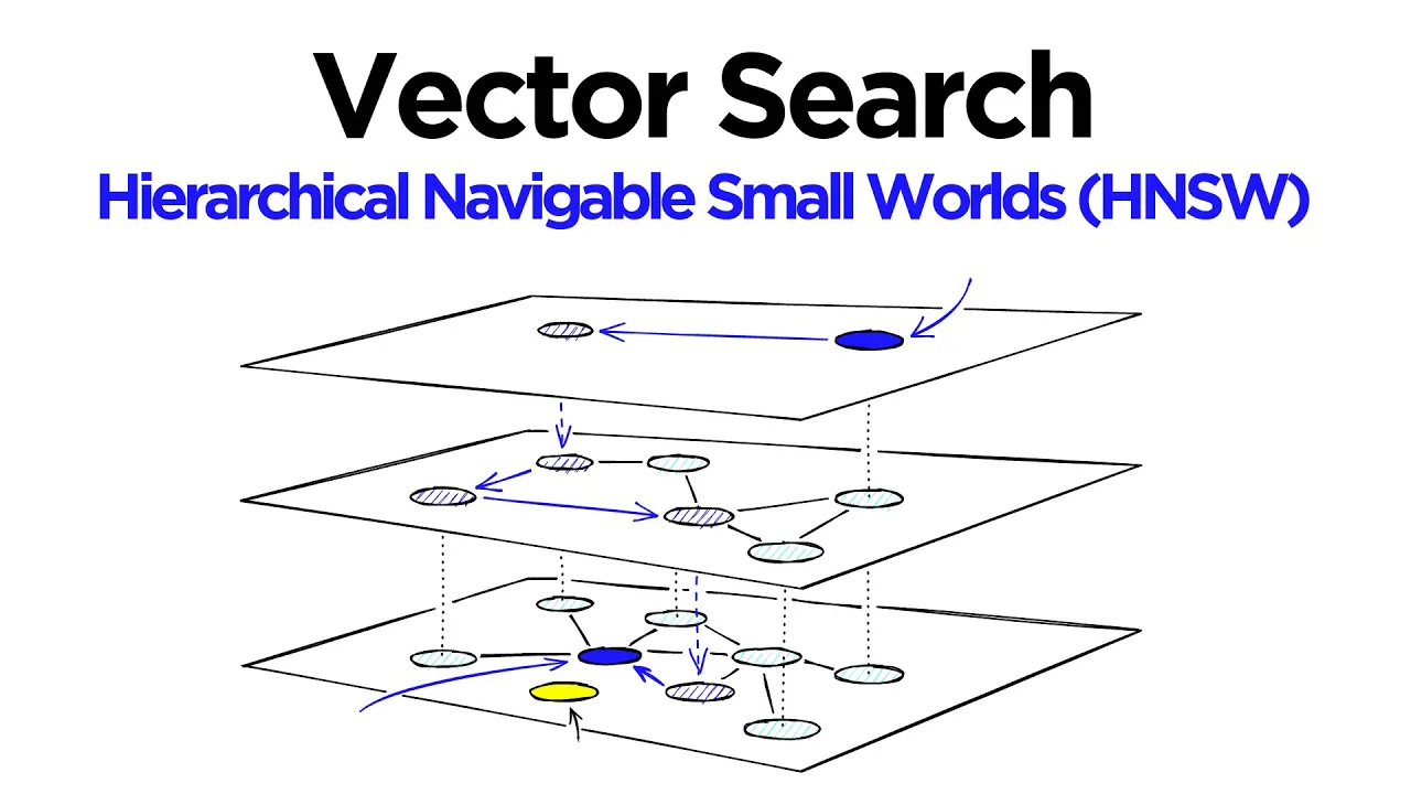
Exploring advanced graph-based index structures such as Hierarchical Navigable Small World (HNSW) for superior search trade-offs.
Deploying vector search in production using dedicated vector databases like Milvus, Qdrant, or Pinecone.
Designing Retrieval-Augmented Generation (RAG) pipelines that integrate FAISS with Large Language Models (LLMs).
Implementing hybrid search strategies that combine dense vector search with traditional sparse keyword retrieval (e.g., BM25).
Scaling similarity search using FAISS GPU acceleration and distributed indexing for billion-scale vector datasets.
85.2K views1.5Klikes31:36Original Release: 2021-07-13
hi welcome to this video we're going to be covering facebook ai similarity search or feis and we're going to be covering what feis is and how we can actually begin using it and we'll introduce a few of the key indexes that we can use so just as a quick introduction to feis as you can probably tell from the name it's a similarity search and it's it's a library that we can use from facebook ai that allows us to compare vectors with a very high efficiency so if you've seen any of my videos before on building sentence embeddings and comparing sentence embeddings in those videos i just did a generic python loop to go through and compare each embedding and that's very slow now if you're only working with maybe 100 vectors it's probably okay you can deal with that but in reality we're probably never going to working with that smaller data set facebook ai similarity search can scale to tens hundreds of thousands or up to millions and even billions so this is incredibly good for efficient similarity search but before we get into care i'll just sort of visualize what this index looks like so if we imagine that we have all of the vectors that we have created and we put it into our our similar search index now they could look like this so this is only a three dimensional space but in reality there would be hundreds of dimensions here in our use case we're going to be using dimensions of 768 so you know there's a fair bit in there now when we search we would introduce a new vector into here so let's say here this is our query vector so x q now if we were comparing every item here we would have to calculate the distance between every single item so we would calculate for between our query vector and every other vector that is already in there in order to find the vectors which are closest to it now we can optimize this we can improve we can decrease the number of dimensions in each of our vectors and do it in a intelligent way so they take up less space and the calculations are faster and we can also restrict our search so in this case rather than comparing every single item we might restrict our search to just this area here and these are a few of the optimizations at a very high level uh that we can do with fives so that's enough for the introductions files let's actually jump straight into the code okay so this is our code in here this is how we are loading in all of our sentence embeddings so i've gone ahead and processed them already because they do take a little bit of time to actually build but we're building them from this file here we'll load this into python as well but i mean it's pretty it's pretty straightforward to say load of sentences that have been separated by a new line character and then here we have all of those numpy binary files now the numpy binary files like i said we're getting them from github which are over here that's where we're pulling them all in using this cell here now that saves everything to file and then we just read in each of those files and we append them all into a single numpy array here and that gives us these 14.5 000 samples each embedding is a vector with 768 values inside so that's how we're loading in our data i'll also load in that text file as well so we just want to do with open sentences dot text and then we'll just read that in it's a normal file and we just write i'm going to put lines equals fp.read and like i said we're splitting that by newline characters so we just write that sorry sentences and see a few of those as well okay now to convert from those sentences into those sentence embeddings i need to import this anyway for later on when we're building a query vector so i'll just show you how i do that now all we do is from sentence transforms which is the library we're using to create those embeddings import sentence transformer and then our model we're using sentence transformer again and we're using the bert and bass lli mean tokens model okay so that's how we we initialize our model and then when we're encoding our text we'll see in the moment we just write model and code and then we write something in here hello world okay and and that will encode that will give us a sentencing embedding okay so that is what we have inside here we just have the sentence embeddings of all of our lines here now i think we have everything we need to get started so let's let's build our first five index so the first one we're going to build is called the index flat l2 and this is a flat index which means that all the vectors are just flat vectors we're not modifying them in any way and the l2 stands for the distance metric that we're using to measure the similarity of each each vector or the proximity of each vector and l2 is just euclidean distance so it's a pretty straightforward function now to initialize that we just write files so we imported now so we need to import files and then we write index equals files dot index flat l2 and then in here we need to pass the dimensionality of our vectors or our sentence embeddings now what is our dimensionality so each one is 768 values long so if we'd like a a nicer way of writing out we put sentence embeddings and we write shape one okay and our index requires that in order to be properly initialized so we do that that will be initialized let me run it again umd i think my notebook just restarted it did restart it's weird okay one minute so that's going to initialize the the index and there is one thing that we need to be aware of so sometimes with these indexes we will need to train them so if if the index is going to do any clustering we would need to train that clustering algorithm on our data and now in this case we can check you know if an index needs training or is trained already using the is trained attribute and we'll see with this index because it's just a flat l2 index it's not doing anything special we'll see um because it's not doing anything special we don't need to train it and and we can see that when we write is trained it says it's already trained just means that we don't actually need to train it so that's good now how do we add our vectors our sentence embeddings all we need to do is write index add and then we just add embeddings like so so pretty straightforward so add sentence embeddings and then from there we can check that they've been added properly by looking at the end total value so this is number of embeddings or vectors that we have in our index and with that we can go ahead and start querying so let's first create a query so we'll do xq which is our query vector and we want to do the model and code that we did before now i'm going to write someone sprints with a football okay that's going to be our query vector and to search we we do this so we write d i equals index search xq and then in here we need to add k as well so k let me let me define it above here so k is the number of items or vectors similar vectors that we'd like to return so i'm going to want to return four so with here with this we will return four index ids into this i variable here i'm going to time it as well just so you see how long it takes and let's print i you see that we get these these four items now these align to our lines so the the text that we have up here that will align so what we can do is we can print all of those out so let's do i and then in here we want to write lines i for i sorry let me end for i in i okay ah sorry so this is zero here okay so these are the sentences or the similar sentences that we've got back and we see obviously it's working pretty well all of them talking about football or being on the on the football field so that looks pretty good right only problem is that this takes a long time we don't have that many vectors in there and it took 57.4 milliseconds so yeah it's a little bit long and something that we can actually improve okay so before we move on to the next index i just want to have a look at sort of speed that we would expect from this when we are this is very small data so what else could we expect so if we go over here i've already written all this code if you'd like to go through this notebook i'll leave a link in the description so come down here we have this flat l2 index and this is the query time so this is for a randomly generated vector with a dimension size of 100 and this is the number of vectors within that index so we go up to 1 million here and this is the query time in milliseconds you can see you know increases quite quickly now this is in fact but it's still an exhaustive search we're not really optimizing how we could do we're not using that approximate search capabilities of files so if we switch back over to files we can begin using that approximate search by adding partitioning into our index now the most popular of these uses a technique very similar to something called vernoy cells i'm not sure how you pronounce i think that's i think that's about right and i can show you what that looks like so over here if we go here we have all of these so this is called a voronoi diagram and each of the sort of squares or the cells that you see are called voronoi cells so here we have voronoi cells and that that is just what you see here so this this you know all of these kind of squares are each a cell now as well as those we also have our centroids so i'm going to write this out instead so centroids and these are simply the centers of those cells now when we introduce a new vector or our query vector into this what we're doing is essentially so we have our query vector and let's say let's say it appears here now within these are on these cells we actually have a lot of other vectors so we could have you know we could have millions in each cell um so there's a lot in there and if we were to compare that query vector and this this thing here to every single one of those vectors it would obviously take a long time we're going through every single one we don't want to do that so what this approach allows us to do is instead of checking against every one of those vectors we just check it against every centroid and once we figure out which centroid is the closest we limit our scope to only vectors that are within that centroid foreign cell so in this case it would probably be this centroid here which is the closest and then we would just limit our search to only be within these boundaries now what might find is maybe there's the closest vector here is actually here whereas the closest vector here is right there so in reality this vector here this one might actually be a better approximation or a better it might be more similar to our query and that's why this is approximate search not exhaustive search because we might miss out on something but that is kind of outweighed by the fact that this is just a lot a lot faster so it's sort of pros and cons it's whatever is going to work best for your use case now if we want to implement that in in code first thing that we want to do is define how many of those cells that we would like so i'm going to go 50 so use this endless parameter and then from now we can sell our quantizer which is it's almost it's like a another step in the process so with our index we are still going to be measuring the l2 distance so we still actually need that index in there so to do that we need to write files index flat l2 and we pass out dimensions again just like we did before and like i said that's just a step in the process that's not our full index our full index is going to look like this so we write index and in here we're going to have our files and this is a new index so this is the one that is creating those partitions so right index ivf flat and in there we need to pass our quantizer the dimensions and also the endless okay now if you remember what i said before we in some cases we'll need to train our index now this is an example one of those times because we're doing the the clustering and creating those foreign cells we do need to train it and we can see that because it's false now to train it we need to just write index train and then in here we want to pass all of our sentence embeddings so sentence embeddings like so let's run that it's very quick and then we can write it's trained and we see that's true so now we can now our index is essentially ready to receive our data so we do this exactly the same way as we did before we write index add and we pass our sentence embeddings again and we can check that everything is in there with index and total okay so now we see that we have our index it's ready and we can begin querying it so what i'm going to do is use the exact same query vector that we used before i'm going to time it so we can see how quick this is compared to our previous query and we're actually going to write the exact same thing we wrote before so you can actually just copy it so take that bring it here there we go so now let's have a look so total 7.22 so bring it up here and we have 57.4 now this is maybe a little bit slow so so you will see that the times do vary a little bit quite randomly but maybe that's a little bit slow but it's probably pretty realistic so that took 57 milliseconds this one seven now let's have a look so these are the indexes we've got let's compare them to what we had before and i believe they're all the same so we've just shortened the time by a lot and we're getting the exact same results so that's pretty good now sometimes we all find that we do get different results and a lot of time that's fine but maybe you know if you find the results are not that great when you add this sort of index then that just means that this search is not exhaustive enough like we are using approximate search but maybe we should approximate a little bit less and be slightly more exhaustive and we can do that by setting the n probe value so n pro uh let's explain a minute so let me actually first just run this and we can see it will probably take slightly longer so yeah we get 15 milliseconds here of course to get same results again uh because there were no accuracy issues here anyway but let me just explain what that is actually doing so in this case here what you can see is a ivf search where we are using an emperor value of one so we're just using we're just searching one cell based on what the first nearest centroid to our query vector now if we increase this up to a or less let's use a smaller number in this example so maybe we increase it to four our four nearest centroids so i would say probably these this one this one this one and the one we've already highlighted all of those would now be in scope because our end probe value so the number of cells that we are going to search is four now if we increase again to say six these two cells might also be included now of course when we do that we are searching more so we might get a better performance better accuracy but in terms of performance in time it's also not it's also going to increase and we don't want time to increase so there's a trade-off between those two in our case we don't really need to increase this so don't really need to worry about it so that is the index ivf and we have one more that i want to to look at and that is the product quantization index so this is actually so we use we use ivf and then we also use product quantization so so it's probably better if i try and draw this out so when we use product quantization imagine we have one vector here so this is our vector now the first step in product quantization is to split this into sub vectors so we split this into several and then we we take them out we pull these out and they are now their own sort of mini vectors and this is this is just one vector that i'm visualizing here but we would obviously do this with many many vectors so that would be many many more so in our case that's 1 15 that just under 15 000.
now that means that we have a lot of these subvectors and what we do with these is we run them through their own clustering algorithms so what we do is we we end up getting clusters and each of those clusters is going to have a centroid so this one would also be run through one so each uh each subset of vector slices is going to run through its own um its own clustering algorithm creating these centroids and these centroids are smaller in size than the the original sub vectors here and what we do is for each of these uh sub vectors so each of these sub vectors they get pulled into here so maybe maybe this one is here and it gets assigned to its nearest centroid and then we take that assignment all the way back over here and add it into add it into our vector so this this is centroid three for example and when i say assign it back it's probably the wrong way to to think about it maybe it's more it's more like this so it becomes a new vector from those centroid ids okay so this would be three now what that does is essentially reduces the size of our vectors but pretty significantly depending on on what dimensions we use there so let's go back to the code let's implement that now we need to define two new variables here so m which is going to be the number of centroids in the in the final vector so [Music] that one thing that we we do need to know with m is that m must be we must be able to multiply m into d so what is our d value it's 100 i can't remember um where are we let me check so 768 now we should be able to divide that into eight i think yeah so this is good we can use eight for m but we couldn't use something like five because if we if we do five we see that d doesn't fit n uh so five doesn't fit nicely into d whereas eight does so m or d must be a multiple of m otherwise we're going to get an error and that's because of the way that the those vectors are broken down into the final centroid id vectors and we also need to specify the number of bits within each of those centroids so this value we can we can use what we want i'm going to use eight and then we can set up our index and also the quantizer so we use a quantizer as we did before so the quantizer is going to be five dot index flat l2 d and also our index here is going to be [Music] so this is a new one this is index ivf pq so it's not a flat vector anymore which is uh the full vector it's a quantized vector so where we have um you know reduce the size of it through this through the method i explained before we drew out now we need to pass a few arguments into here first one is the quantizer so the quantizer d which is our dimensionality endless m and bits so pass all those to our index uh sorry we need five there as well and there we go so we we now have our index again you may guess that we might need to train this one there we go so to train it we just write index.train that's our sentence embeddings okay so might take a little bit longer this time there we go and then we can we can add our vectors now after adding those let's see how quick this is should be a lot quicker or a fair bit quicker it's hard to get much quicker and less on so we're going to use the same codes before so i'm going to take this right down here see 2.86 so yeah we've gotten a lot faster so we've gone from what was up here 57 milliseconds and down to two now there is one thing here these these values are now different so that's a the accuracy has has decreased so if we where is the last one here so you can see that we are getting so we have the 190 we still have that one and we have the 12 465 but these two at the front are now different and this is just you know it's on the trade-offs of accuracy versus speed so if we come down here let's well let's give that a go let's uh let's have a look at what we are pulling through so i'll copy this again and let's just see so we have these i mean although the the accuracy has decreased technically because it's not getting the same results as the exhaustive search there's still pretty good results so i mean nonetheless i think that is pretty cool so let's have a look at let's compare this to our previous two of the methods in terms of as we did before the graphs so here is that final one so we have ivf pq along the bottom yeah it's a lot faster right um and then we have ivf flat with a n-prime value of 10 much faster than l2 but still not quite as fast as as pq and then and then we have flat or two at the top which obviously much so and just as well just be aware on the left here we have the we have a log scale so the differences are pretty pretty significant when we go to the one million mark so i think i think that's it for for this video so i think obviously fires is pretty cool definitely really useful and i think we're definitely going to explore it more in in the future so for now that's it so thank you for watching and i'll see you in the next one
Up Next

21:14
ChromaDB Vector Database Guide: Embeddings, Semantic Search, RAG
@alejandro_ao
5.1K views•2025-09-29
87:26
Introduction to Secure Multiparty Computation with Yehuda Lindell
@fhe_org
7.7K views•2021-02-04
34:35
HNSW Vector Search: Implementation with Faiss in Python
@jamesbriggs
50.3K views•2021-10-05

19:25
Enigma Machine Mechanics: WWII Encryption Explained
@JaredOwen
13.2M views•2021-12-11
Related Study Plans & Knowledge Roadmaps
Structured learning paths in Computer Science
computer-science
Container Runtimes: Namespaces, Cgroups & Go
01Linux Systems & Go Programming Foundations
02The Core of Isolation: Chroot and Filesystems
03Linux Namespaces: Process Isolation
+ 3 more learning modules
32h6 modules
Explore Roadmap
computer-science
Building a CHIP-8 Emulator: Rust & CPU Basics
01Computer Architecture Foundations (Bits & Bytes)
02Rust Programming for Systems Development
03CHIP-8 Virtual Hardware Specifications
+ 2 more learning modules
32h5 modules
Explore Roadmap
computer-science
Building BitTorrent: Go, P2P & Concurrency
01Go Fundamentals & Concurrency
02Networking Foundations & P2P Architecture
03Bencode Parsing & Torrent Metadata
+ 3 more learning modules
26h6 modules
Explore Roadmap
computer-science
Actor Models (C++ Concurrency & Lock-Free)
01C++ Multi-Threading Foundations
02Thread Pools and Task Scheduling
03Atomics and Lock-Free Queue Design
+ 3 more learning modules
45h6 modules
Explore Roadmap