






![[머신러닝+딥러닝 기초 강의] 22강. 합성곱 신경망의 시각화](https://i.ytimg.com/vi/28beETw65Ec/maxresdefault.jpg)









![Adam Gleave – Will Scaling Solve Robustness? [Alignment Workshop]](https://i.ytimg.com/vi_webp/kqDEkzSbwwo/maxresdefault.webp)








This lecture from Stanford's CS231n Winter 2016 course covers multiple techniques for understanding and visualizing CNNs, including examining raw activations, visualizing filter weights, using t-SNE for dimensionality reduction, conducting occlusion experiments, and employing optimization-based methods like DeepDream and neural style transfer. The lecture explains how guided backpropagation improves visualization quality by filtering out negative gradient influences, and discusses adversarial examples that demonstrate CNN vulnerabilities when small input perturbations exploit the linear nature of network functions.
CS231n Lecture 9: Visualizing CNNs, Deep Dream, Neural Style & Adversarial Examples
Added:Fundamental understanding of Convolutional Neural Network (CNN) architectures, including convolutional, pooling, and fully connected layers.
Familiarity with backpropagation and gradient-based optimization algorithms used to train deep neural networks.
Concept of feature representation in deep learning, specifically how early layers capture low-level features and deeper layers capture high-level features.
Basic knowledge of loss functions, such as cross-entropy loss, and how they direct optimization.
Generative Adversarial Networks (GANs) and Variational Autoencoders (VAEs) for sophisticated image synthesis and generation.
Adversarial defense strategies and robust training techniques to secure deep learning models against adversarial attacks.
Explainable AI (XAI) and interpretability frameworks (e.g., SHAP, LIME, Integrated Gradients) for auditing complex black-box models.
Real-time Neural Style Transfer techniques and feed-forward style transfer networks.
Advanced computer vision tasks such as object detection and semantic segmentation (e.g., YOLO, Mask R-CNN) which build upon feature visualization principles.
66.4K views535likes1:18:20Original Release: 2016-02-04
So today we'll talk about uh understanding and visualizing convolutional neural networks. This is one of my favorite lectures to give because we'll get to look at a lot of pictures, videos, have a lot of fun and there's a lot of space for kind of intuitive understanding of what cometets are doing. Before we dive into it, just some of the administrative items. Um assignment one is now now graded. We'll send out the grades tonight. I'm saying or so because just in case that something goes wrong and we can't find a way to send it out to you. Uh but uh definitely we'll try to have it out by tonight. Assignment two, just a reminder, is due this Friday. Uh you have to submit it differently from last time. So last time you submitted on the Dropbox in coursework. This time please submit in an assignment tab. That's a difference from last assignment. Uh so for assignment two, submit it in the assignments tab. And as a reminder, midterm is next week on Wednesday. And so I posted some information on the piaza about the midterm and the sample midterm as well. Oh, and some uh small fun piece of news is that ResNets uh the winning models from 2015, the large 152 layer model is now um has now been uploaded. The weights have been uploaded to uh to GitHub and so you can use these models now in your projects if you like.
So this is a cafe model, but I think several other packages should be able to load it as well, but we're not 100% sure about it. So you have to check it out.
Um but yeah, so we're talking about convolutional networks. We saw that connets are useful in a wide variety of application domains. Uh in two lectures ago, we saw uh how convolutional networks work. So we have these com pool fully connected layers. We're stacking them up into architectures. We looked at all the winning architectures over the last few years and you got a sense of how we actually wire up comnets to to get uh award-winning performance. Um and then a lecture ago, Justin was talking about object detection localization. So um in this case we looked at RCNN fast RCNN faster RCNN YOLO and really how you have this idea of multiple heads on top of a comnet. So some heads are doing classification, some heads are doing regression and they're trying to just localize all these things in images in various ways and we looked into that. So this lecture is mostly about understanding and visualizing. So we'll look at various uh ways in which we can visualize how comnets work. So you run a comn net on imageet and you see that your performance is say 5% top five error and you can tell that it's working very very well. But exactly how does this performance come about and how can we study it or understand uh what's happening. So we'll go through several of these. I think we'll spend most of the time on the very last one. So I'll kind of like breeze through some of them um some of the earlier ones. So probably the simplest way to actually understand what comes might be doing is to look at the raw activations of a comnet. So in a convolutional network we pass in the image at the bottom. we get all of these different activation volumes in between and at the end we have a classifier on the top. So one of the ways you can study what these connets are doing for example is we can pick on an arbitrary neuron say in a pool five layer and we can pipe lots of images through comnet and just see what excites that neuron the most. So then you get visualizations like this where for example every row here corresponds to a neuron and every single image here is something that excites that neuron a lot based on the entire training set of imageet. And so you can see that some neurons basically they like spotlights either on a person's forehead or just in general. Uh some neurons are more interpretable than others. So some of them like text and some of them like dogs or American flags. So it's not clear exactly what's going on. So not all of them as interpretable as as others but it kind of tells you something a bit. Another way we can study this is not just looking at the activations but looking at the weights and in particular we saw that we can look at the first convolutional layer in the comet and these uh this first convolutional layer consists of a filter bank of filters that we slide over the image and so we can visualize the raw filter weights. Um and we can see that the comet on the very first layer is looking at all of these different rotated gabbor like features as we like to call them. Now the problem with this visualization of course is that this only makes sense to do on the very first layer where you actually have contact with the raw image. But for the other convolutional layers they're looking at the convolutional layers below and so their weights are not very interpretable. So you can still do it. Uh so for example in my coms demo I still visualize the weights of higher convolutional layers.
So in the first layer you can see com one filters and they make sense. The second one is a comp 2 filter bank. And every single array in brackets corresponds to a single kind of filter or kernel. And you can see that there's some structure to them, but it doesn't make too much sense. It's not very easily interpretable because these act over activations on the previous com volume, not on the raw image. Uh so this doesn't make as much sense and it's not as um as nice to look at. Now you might think that for example, the fact that this emerged just from training is amazing that you can get these gabbor like filters out of these networks. It turns out that there's actually it's not actually true um in a sense that there's a bit of a there were many papers uh that were written before comuts where there's many different unsupervised and supervised objectives you can come up with and pretty much anything you throw at an image where you're trying to learn a feature with different algorithms you almost always achieve these gabbor like filters. So it's not super exciting. Uh there's a bit of a fatigue about it but uh but basically um I just wanted to point that out as kind of like a fun aside. In fact, the converse is true. It's hard to come up with a reasonable algorithm that does not give you gabbor filters on the first layer. U I think the only example I'm familiar with, for example, is PCA. It doesn't give you gabbors. It gives you these kind of wave sinosoids and so on.
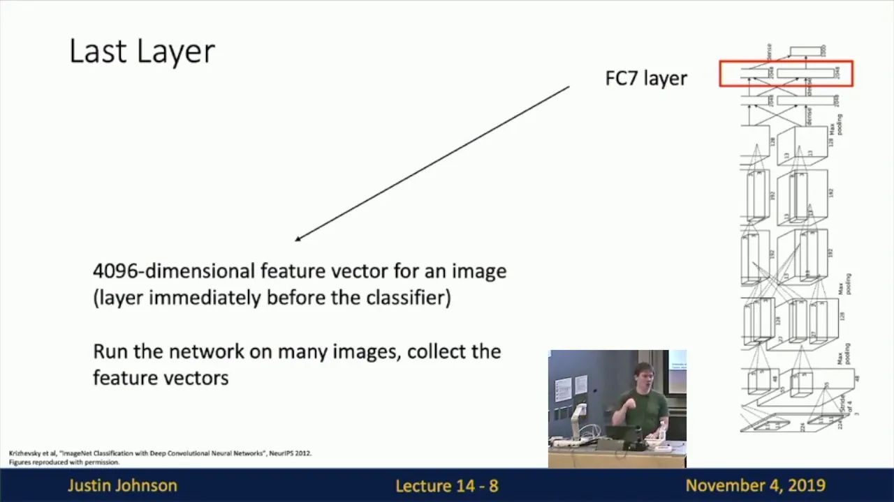
But anyways, um so another way to study comets is in this more global representation kind of view. So we looked at filters, we looked at the weights. Another way to study this is we can take a lot of images through a comnet and we can look at what I refer to as FC7 features or codes or something like that. Um, and there's 4,96 numbers just before the classifier, right? And so we can interpret those 496 numbers as summarizing the content of the image. And so we can think of these as codes. And so lots of images as we put them through, we get 4,96 numbers for each one of them. And we have a large collection in this 4,96dimensional space. And now one way to visualize this uh is for example using something called tney visualization. I won't go into details how this works but it's something that every one of you should be familiar with aware of that should be in your toolkit. It's very it makes very nice pictures. Intuitively what tin does is you give it a collection of highdimensional vectors and it finds an embedding in two dimensions such that points that are nearby in the original space are nearby in the embedding and it does that in a particularly clever way um that actually gives you very nice looking pictures. So here for example is the mnest data set of digits uh which are 28x 28 images. So this is I think 768 dimensional vectors and they're embedded in 2D and you can see that the digits from 0 to 9 they kind of cluster uh in this visualization. So we can run tney on codes of images in imageet and when you do that you end up with some nice visualizations. Um, so what what I've done here is I take all the codes and I embed them and whatever is close in this visualization is basically close in the mind of the network. You can sort of look at it that way. So there's lots of embeddings here on this website. I pre-loaded some of it. Um, so this is in a raw space and then these are some visualizations where I've actually like warped out the representation to make it a square. And then here's actually if we try to zoom in. Um, so these are all anything that's nearby is basically very similar looking to the comnet. And so you can see all the headlights kind of cluster here, keyboards, all the circular things.
Um, then we go down, all the spaghetti, uh, mushrooms. Um, there's a cluster on the on the right here. That's all the dogs are, all the animals in general.
Some people cluster in the middle here.
Uh, boats, I don't know. So random things basically they cluster in very interesting way. Um and so that gives you an idea about what come considers to be uh similar to each other. So you can go through these they're fun to look at.
So that's tne. How about different types of objects? How are they, you know, why are they close to each other? Um why are they close to each other? It's a I guess it's a very good question. So a connet has to classify all these different 10,00 categories, right? And it only has a finite capacity uh to do that. And so it ends up um in its process of trying to find the best ways to fit the data, it just ends up uh transforming transforming your images into some kind of a nice dimensional space where it's easy to classify them. And this is a visualization of that space. So I I can't say much more than that basically.
Uh so that's uh TC visualizations fun to look at. Another kind of uh fun experiment kind of on the side um that you might want to maybe perform in your projects maybe. I'm not sure uh is occlusion experiments which are kind of fun and give you some idea about what comes might be doing. What we'll do here is we'll take an image like the one on the top there and the conet classifies it as a Pomeranian. It's a specific type of dogs a dog. And now what we'll do is we'll have a patch of zeros that we're going to slide through the image and olude part of the image. So there's an occludder here in gray. It's kind of difficult to see this occludder patch and we'll slide it spatially through the image. And as we do that, we are looking at the probability of Pomeranian and how it varies as a function of the spatial location of that occludder. And so we're going to carve out an activate a kind of a heat map here of uh what happens to the probability of Pomeranian as you slide this through. And so what might you would expect for example from this kind of visualization? What would be nice a nice result? Um yeah, go ahead. When you cover up the face of Yes. So you'd like So when you cover up the face of this dog, you'd like maybe the property to go down. So that's in fact basically what happens and so what you see is the comet doesn't care if you occlude any of these regions but when you occlude the face of this dog suddenly the probability of pomeranian plummets and so that gives you some confidence that basically this is the features that really matter in the prediction and it's actually looking at the dog. Uh if you do the same here for carwheel then carwheel is the region where your probability plummets. Uh for this Afghan hound if you olude the dog then you go down to uh the probability goes down by a lot. Interestingly, in this picture, by the way, if you olude the person's head, then uh basically the probability actually goes up. So, it's kind of like the combinant is not really sure if there's a class here, like maybe there's some class related to a hat on a person or something like that. But once you include that region, the com becomes more certain that actually afghan hound is the class for this image. So, that's kind of interesting. Um, okay. So, that's kind of on the side a few things that I kind of marched through as a bullet points.
We're now going to go into uh two more types of visualizations. And I'll actually show you this video. I'll actually play the 4-minute video in a second throughout this video because it's a very good video by Jason Yosinski. Um, and he has this toolbox called deepb this toolbox and you can download this code then you can run it and what it's doing as you'll see is it's running net in real time and you can sub in your camera feed and you can play with the comnet and see all the activations and throughout the visualization he'll be showing some he'll be showing two separate kinds of visualizations for neurons. One is um decomv and the other is optimization based and we'll cover those later in the class but for now I guess uh these kinds of pictures you'll see them. We'll cover them in a bit. Let's look at the video.
It's a fun video.
Recent advances. Oh shoot. I didn't fully think this through. How do I get uh lots of volume here? Not actually even sure if Okay, we have to be very quiet. Basically, recent advances in neural networks have enabled computers to better see and understand the world. They can recognize school buses and zebras and can tell the difference between Maltese terriers and Yorkshire terriers. We now know what it takes to train these neural networks well, but we don't know so much about how they're actually computing their final answers. We developed this interactive deep visualization toolbox to shine light into these black boxes showing what happens inside of neural nets. In the top left corner, we show the input to the network, which can be a still image or video from a webcam.
These black squares in the middle show the activations on a single layer of a network. In this case, the popular deep neural network called Alexet running in cafe. By interacting with the network, we can see what some of the neurons are doing.
For example, on this first layer, the unit in the center responds strongly to light to dark edges. Its neighbor one neuron over responds to edges in the opposite direction, dark to light. Using optimization, we can synthetically produce images that light up each neuron on this layer to see what each neuron is looking for. We can scroll through every layer in the network to see what it does, including convolution, pooling, and normalization layers. We can switch back and forth between showing the actual activations and showing images synthesized to produce high activation. We'll go into this in a bit.
By the time we get to the fifth convolutional layer, the features being computed represent abstract concepts. For example, this neuron seems to respond to faces. We can further investigate this neuron by showing a few different types of information. First, we can artificially create optimized images using new regularization techniques that are described in our paper. These synthetic images show that this neuron fires in response to a face and shoulders. We can also plot the images from the training set that activate this neuron the most as well as pixels from those images most responsible for the high activations computed via the deconvolution technique. This feature responds to multiple faces in different locations.
And by looking at the decom, we can see that it would respond more strongly if we had even darker eyes and rosier lips. We can also confirm that it cares about the head and shoulders, but ignores the arms and torso. We can even see that it fires to some extent for cat faces. Using backcrop or decon, we can see that this unit depends most strongly on a couple units in the previous layer con 4 and on about a dozen or so in con 3.
Now, let's look at another neuron on this layer. So, what's this unit doing?
From the top nine images, we might conclude that it fires for different types of clothing. But examining the synthetic images shows that it may be detecting not clothing per se, but wrinkles. In the live plot, we can see that it's activated by my shirt. And smoothing out half of my shirt causes that half of the activations to decrease. Finally, here's another interesting neural. This one has learned to look for printed text in a variety of sizes, colors, and fonts. This is pretty cool because we never asked the network to look for wrinkles or text or faces. The only labels we provided were at the very last layer. So, the only reason the network learned features like text and faces in the middle was to support final decisions at that last layer. For example, the text detector may provide good evidence that a rectangle is in fact a book seen on edge. and detecting many books next to each other might be a good way of detecting a bookcase, which was one of the categories we trained a net to recognize. In this video, we've shown some of the features of the deep viz toolbox and a few of the things we've learned by using it. You can download the toolbox of this URL and explore for yourself. If you'd like to share what you find, you can use the hashtag deep viz. Thanks for listening and we look forward to seeing what you discover.
Yep. So, that's deep viz toolbox. Pretty cool. Um did you guys hear it by the way? Was it okay awesome? So that's pretty cool, right? So you can investigate these kind of and debug them in real time. So two kinds of visualizations again that he presented there are um decompased approach and optimization based approach and we'll go into those now uh one by one. So I'll show you first how we generate some of the decom images that he showed.
Um so before we actually dive into it, I'd like to kind of start off with a question. Um suppose I feed an image through a convolutional network and we get all these activations throughout.
Think about how can you compute the gradient of any arbitrary neuron in the network with respect to the image. So in other words, the gradient on the image for any arbitrary neuron in the network is computable. Of course, it's a smooth function because the comnuts are a differentiable function. Uh but how would you actually compute that in in a codebase? Like say you're working on your assignment and you have your forward backward your layers. What is a practical easy way to actually compute this gradient with respect to any arbitrary neuron. So normally what we're computing gradient with respect to is we have this entire computational graph where we pass the image through and we get a loss at the end and then we uh if you remember your computational graphs um your computational graphs we we start off the back propagation by setting a 1.00 0 0 gradient there because we want the gradient with respect to loss with the gradient of the loss with respect to loss is once upon zero and we run back prop backwards and find the influence of all the inputs on that output. So how would you do it now if you wanted a specific unit in the comnet and find gradient for it? Back prop from there.
Back prop from there. Okay. So we do a forward pass and then suppose we're interested in some layer and that neuron. What would you do?
Stop there and back prop. Just stop there and back prop. So you have to start off with like some gradient, right? So what we'll do is we forward until some layer and then we have our activations at that layer and now we're interested in some specific neuron.
We'll zero out all the gradients in that layer except for the neurons gradient.
We'll set that gradient to 1.00 and then we run backward from that point on. And then when you backrop to the image, you'll find the gradient of the image with respect to any arbitrary neuron by meddling with the gradients. And so in particular, we want to set the gradient of the one we're interested in to be 1.0. And so yeah, why why don't we just use like numerical gradient compared to the gradient? Um why don't we just use the numerical gradient? Because it's just slower, right? So we we could use a numerical gradient to also compute uh the gradient with respect to any arbitrary part of the network but it's just you'd have to iterate over all the pixels one by one and it would just be slow. So this way we can use the analytic gradient right we're just doing back propagation and just computing it uh right away using calculus. So for example if we wanted gradient not with respect to the loss function but in this computational graph we wanted the gradient for this guy here this gate then what I would do is I would run the inputs forward until this gate and then I would stop right there and I would just set 1.00 0 0 as the gradient at this point and I would just run back propagation from here and whatever gradients I obtain here are the basically gradients the influence of these neurons on this guy. So that's how you can compute um your influence on any arbitrary part of the network.
So when you do that with an image, you uh suppose we wanted to like pick on an arbitrary neuron, you take an image, you forward it through, and you do what I described. You set the gradients to all zero except for neuron you're interested in, and you run backward for them from there. And you'll find, for example, looking at an arbitrary neuron, you'll find some something like this as the gradient on the image. So you can see that it's not very easily interpretable.
It's kind of like these blobby things.
Looks kind of strange. So decom approach uh will change the backward pass a bit uh to actually give us nicer pictures.
So in this case for example we'll use what's called guided back propagation and we'll actually obtain much cleaner images of say this cat's head specifically. So that neuron would be looking would be positively influenced by this cat's face specifically and we'll see how we can get rid of these artifacts. And so the way this will work this decom approach works is I'm going to go through a figure from the paper.
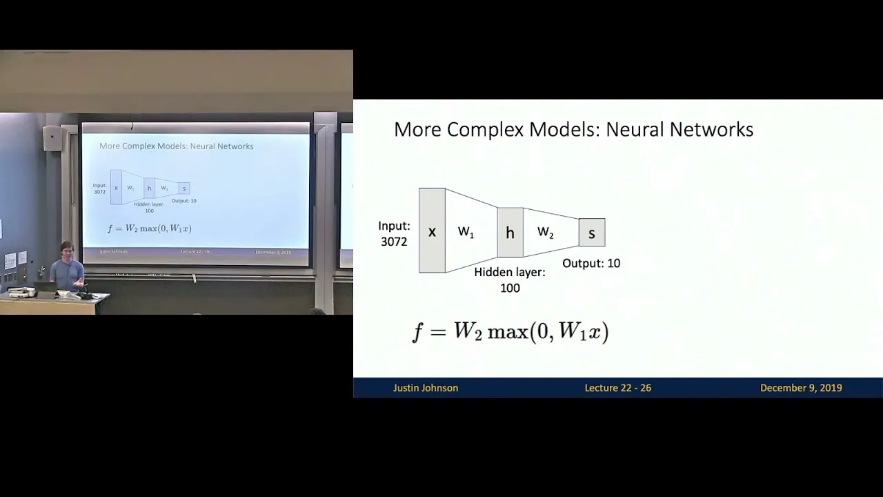
Uh this is striving for simplicity paper. uh so I have to explain this a bit. So here we have the input image goes through a series of layers and we get some activation feature map at some point in the comnet. And now as I mentioned if we'd like to derive the gradient for for any arbitrary neuron here say like this neuron in the bottom right we'd zero out. So these are the gradients. Now in this second row here we'd zero out all the gradients except for that neuron and we do back propagation to find the reconstructed image as they call it. But really it's it's the backward pass here. Now, when we're doing back prop, um it turns out that to get your decom approach to give you nice interpretable pictures, we're going to be running back propagation just like um in a previous slide, but we'll um we'll meddle with the back prop for specifically the ReLU layer. Uh so the ReLU layer just uh thresholds things at zero. We we'll change the backward pass for a ReLU layer and otherwise we'll run backward through the image and I'll you'll see in a bit why that kind of makes sense. Um so we're looking specifically at a rel layer here and what it computes during the forward and backward pass during backward propagation. So if we're in some feature this is some feature mapping net and we apply the relu operation which is thresholding all the negative activations to zero. Now in the backward pass this relu layer finds what the gradient from above is. So this is the gradient going into the re neurons and the way re works right is it just kind of blocks all the gradient for all the parts that had negative activations right because if you're a rel neuron and there's a grid of 3x3 of them here if you're a real rel neuron then if your input was less than zero then you act as a switch during the backward pass right so if gradient comes from here if you're a real neuron and your input was less than zero then you block the gradient and if it was greater than zero then you let the gradient pass through so basically That's what's going on in the backward pass here. So this is just back proposition right now. And this is how you'd write it out. So basically the backward pass for this real neuron is the local gradient which in this case is just a greater than zero operation and then times the gradient from above. So this is the chain rule going on here. How you back propagate through ReLU. Now in guided back propagation what we'll do instead is we'll change the ReLU layer backward in the following way.
we are computing what we had before. So relu pass but in addition we have this additional term here which basically is saying that we only back propagate through our real neurons only the activations only the parts the real neurons that have positive gradient. So okay so this is the guided backdrop. So normally we pass through any gradients that corresponded to real neurons that received less than zero input. And now for gadget backdrop, we're additionally going to block out all the gradients that correspond that are negative gradients. So for example, some of these gradients that ended up passing through this red layer in a backward pass were like -2 or negative 1 or negative one here. We're actually going to kill those. We only backdrop the positive gradients. And so what's going on here is think about the interpretation for what means a positive or negative gradient. In this case, we're trying to compute the influence on the input from the input on some arbitrary neuron in the connet. And what a negative gradient is saying is that this rel neuron has a negative influence on this neuron that we're trying to find what activates it highly. And uh and this is this this piece here has a positive influence and these guys have negative influence and so on. So we're doing is as we're recursing this relu modified rel neuron throughout the comnet which is made up of this comu comu blocks we only end up passing through gradients that have a positive influence entirely positive influence on the activations without the negative influences. So normally what happens is through the comnet this gradient signal is flowing backwards through many relu layers and there are all these paths of influence between the input to any of the output neurons that we're trying to compute and some of the paths are negative paths and some of them some of them are like positive influences and this gradient signal is really just neurons communicating to each other what should increase or decrease and they're kind of fighting each other and adding up and so on. And so what ends up happening with back propagation is the reason you get weird looking things is that you have all these passive influence, some of them positive and some of them negative from every single pixel to the neuron we're trying to u see what activates it. And they kind of end up canceling out in a weird interference pattern. And so what we're doing in guided backdrop is we're only keeping the positive influences and only back propagating those through. And then you end up with much cleaner images. So what this is saying is that this pixel there's a chain through the comnet of positive purely positive influences and there's a very direct uh kind of increase entirely increasing chain of um influences through the comnet on the neuron that you're trying to compute intuitively. Uh go ahead questions. If theation kernel had negative entries then this is not true. Uh sorry if the convolution kernel has negative entries then if we have negative it might be turned into yeah so when you think about a com it's a stack of com relu and so on to first order approximation here we're only changing the relu activations. So in between every relu backward there will be a there will be a a convolutional layer backward and that contains some positive and negative weights and so you end up with some positive and negative uh gradients on the next relu layer but then we again chuncate we throw off all the negative influences again and so we keep doing this recursively through. Go ahead. If you did the opposite and only kept the negative gradients would you get a map of the strongest inhibitory features?
Yeah. So the question is if we only kept negative gradients instead do we get a map of negative inhibitory features? Uh I guess so. Yes. I I've never tried that. It's a good question.
Okay. Oh, was there a question? You're basically just applying Reu backwards.
Yes. So, we're doing backdrop just like everything is normal, just normal backdrop, but you have to hack the Reu backward pass. And in that Re backward pass, you don't just do what normally a ReLU neuron wants to do according to backdrop, but you make sure that you only back propagate to positive gradients through ReLU. So could you use different activation function like instead of using like a instead of just taking positive taking only very large positive or reasonably large positive values I see like if this was not just a relu but say arbitrary neuron I think uh yeah we'd have the same kind of effect if it was 10h or something like that you'd do the same thing and so what ends up happening when you do this is you just get a much cleaner you don't have all these positive negative paths like fighting each other in a way and you only end up with kind of like these positive influences through the network that ends up getting paint painted and So um these are the kinds of visualizations you can get for different neurons. Every row here is a neuron and this ends up uh this is I think com 6 and com 9 uh respectively and uh these are kind of um we forwarded some image through we found that this neuron activates and then we did this backward pass but this hacked up backward pass using the hacked up Reu neuron and these are the kinds of visualizations you you obtain. And so there are kind of this um you can see that some neurons are basically and this is also showing the raw images cropped to the part of the image that uh this neuron is a function of right because these neurons are arranged spatially and their area of influence is different in the spatial image. So these are little crops from images uh which come from the part of the image that activates this neuron. So you can see that some neurons uh these are the raw patches that activate them that activated them strongly and this is the kind of decom pass from her from here. Now there's another way to do it uh not just uh this approach proposed in this paper but there's also something called a decomn net. This is from a paper from Matthew Zyler in 2013 and it it hacks up in the re backward pass as well but in kind of a more funny way. it ignores the relu gradient and it's just passing through the positive gradients uh without without it doesn't care if the activations coming into the relu are positive or negative. It discards that term and so you can see that backdrop a decom and a guided backdrop is kind of both of them at the same time. So it's kind of funky stuff going on but u but for decomn net that turns out to actually also work well and uh and then you get also pictures that actually seem to make sense. So in these cases it's a similar kind of idea to a um to the guided back propagation but um we're not taking into account just like subset of neurons based on what happened to activate in the forward pass. So I don't know if I have very good explanation beyond this point but basically it produces much cleaner pictures because we were only passing through the positive influences entirely positive influences through the backward chain.
Um so these are some uh visualization for the first layer for the second layer. Uh so we can see that some neurons here activate for different kinds of textures. If we go deeper into the network we start to see that on the third layer we get neurons that uh respond to some kind of like honeycomb shapes or um cars or yeah lots of interesting pieces here. And as you go to the fourth layer we start to get some object- like things. So say dog faces here um and so on. And so we're building up these features one at a time. So every comp is kind of combining these little pieces into a higher layer of abstraction kind of shape that grows over time. Go ahead. Why are we considering the gradient? I mean what's the intuition behind looking at the gradient? Yeah. So what this is telling you the gradient really is telling you like the the reason that we see say red here in in this uh person here.
Yeah. like that gradient is telling you that if you were to make this person's face redder, there would be more red in it, then that would have a locally positive influence on this neuron's activation. So basically making a small step in the image in this direction would have um would have positively influenced that neuron downstream, right? That's what the backward pass is telling you. It's telling you that's what back propagation is doing is it's computing the influence the gradient of every single input to whatever you're interested in. Right? So um but in backward pass you have all these positive negative influences and here we're cropping always the negative influences. So you end up with like a subset of the back prop pass almost. You can look at it that way. Um okay so I'm not a huge fan of the decom visualizations. We're going to go into the optimization based uh visualizations which I think make much more sense and are much more intuitive in terms of what's going on. So let me get into those. Uh what's nice about the deco approach is that you do a single forward pass, single backward pass and you're done. you just visualize that hacked up gradient and you get some visualization that looks pretty. In the optimization um approach we're going to have to do a bit more work computationally but it makes a little more sense I think. So what we're going to do here is we're going we have a comet and of course everything is fully differentiable here and what we're going to do now is we're going to try to optimize the image so that we're so the parameters of our optimization now will be image and we'll be keeping the entire comnet fixed. Normally we optimize over the parameters in comnet. Now we'll hold everything fixed and we're going to be trying to maximize an arbitrary score in the comnet. So optimization problem wise basically we're trying to find an image I such that your score is maximized and there's some regularization on I. So say L2 regularization which doesn't u which uh discourages kind of these pathological cases where some of the pieces of your input might be way too large or something like that. So it's regularization and we're trying to maximize the score. And so the way this will work is we'll start off with say like a zero image. We'll feed it into a comn net and get some uh scores out. And now in terms of the gradient again as before we're interested in some class score. So we set the gradient at that point to be all zeros except for a one at the score that we're interested in.
And then we're going to do backward pass to find what change to make to the zero image. So this is normal back propagation. Now we're not doing any more guided or anything weird with relus. This is just straight up back prop. So forward. Now we are interested in some particular gradient signal because we want to increase some score.
We do backward and we do updates. So we're going to iterate this over and over and we're going to basically run optimization over the image to maximize a class score. Uh subject to also a regularization penalty. Okay. So when you do this the kinds of results you get and we're doing updates on this image.
So we're doing image updates instead of the weight updates. Uh you get images like this. So here we are maximizing any class here and these this is the maximally this is the image that maximally activates that class's score.
So we have dumbbells and cups and dalmatations. You can see all the little structured patterns there. It's kind of fun to look at. Ballper lemon husky.
Here we have and also notice for example here's goose. You can see that the the optimization is really trying to take advantage of all the area it possibly has to increase the score of goose. So it like tiles the entire input with goose everywhere because it's just like trying to blow up the score of goose. Um so one goose is good but 10 goosees is much more likely goose. So that's why that happens.
Um one interesting another kind of interesting uh way of interpreting uh the gradient signal at the at the image.
Uh and one way you can use it in an interesting way in this paper from uh Kieran Simmonian is as follows. Um they have this these fun experiments where they take an image like say this dog and they forward the image through the comnet and then they it says that this is some kind of a special terrier or something and then you uh set the gradient for that terrier to be one and you do backdrop and um you arrive at your image gradient and then what they do this is kind of a confusing notation here but they they squish it through channels with a max. So basically they're trying to compute a heat map here, a one-dimensional kind of map of these gradients. And so what might you expect or what would you hope or maybe happens in terms of what this might look like? We're visualizing these gradients.
High on the object location. Okay. So you'd expect that it's high on the object location. I guess that's reasonable, right? So basically this is what happens. So you end up with something roughly like that. um where the gradients the max of the gradients without um taking into account that sign is uh are these blobby things. And so really the way to interpret these maps is it's strength of influence of every single pixel on the score. So the fact that some of this stuff is black, what that's telling you is that if you wiggle that pixel, the score of that dog is basically not modified at all. So the content doesn't care about it. But if you start to meddle with the pixels on the dog, then it's going to actually influence the score in some way of the dog. And so this is kind of telling you area of influence in the image. That gradient signal can be kind of used as a measure of area of influence of every single pixel in the score. Go ahead. So with the slide before you start and you arrive at some optimal image, I was just curious how sensitive is that to choice image? Like if you instead started with random image and optimize that. Uh yep.
So you're asking how sensitive is are these optimizations to the initialization? We'll see actual examples of that in like two slides.
Yeah. Oh yeah. And also with the previous one rather than having like that ridge regression term on there, why don't we just um like put a hard match like 255 or something like that more of a Yeah. So you're asking about the precise forms of regularization used here and the fact that you could use multiple. There's in fact a paper we'll go into in five slides where they actually talk about this regularizer quite a bit more and you want to choose it properly and there are multiple choices here. So what's interesting here is they have these experiments in the paper where you can actually use that gradient and you can use a grab cut segmentation algorithm which we won't go into but that is the input to grab cut and basically grab cut does this joint optimization over pixels and uh you basically want similar pixels or nearby pixels to have the same label and you can actually crop out some of these images just based on the gradient signal uh on the raw image. And so I should like to say that um these are kind of I think I suspect cherrypicked examples uh in this paper because I think we tried it in some of our stuff and that you don't always get this nice uh looking things but uh but in principle you can imagine that this might work sometimes.
Um okay so right now we were maximizing I was showing you examples of maximizing the full score and we were doing optimization of the image and the point here is that you can actually do this for arbitrary neuron in the comnet we saw this with demp as well and so the way this would work is u again we have an optimization over not just the score but maybe any arbitrary activation of any neuron in the network and there's this penalty L2 that we've been using so far in this paper from Jason uh Jason Yosinski they argued that actually there are better ways of regularizing and they were looking for different ways of regularizing the image to make it more image- like and they actually found a different kind of more explicit scheme that they found work better and we'll see uh another set of visualizations that make everything look a bit better I think and the way they do it is they ignore this penalty instead they just maximize and neuron but after they do forward and backward they do an update and then they blur the image a bit so if your image here is X they do forward backward they do a small update on the image and then they blur it. And so this blurring that you keep doing at every single iteration. It's kind of like uh preventing the image of accumulating high frequencies not through the loss function that you're optimizing here.
Although I think you can reexpress it as the blur kernel here corresponding to some total variation loss function but they do it more explicitly like just a blur and then they do a bit more sparsely encouraging things that I don't want to go into. You can check the details in the paper but basically end up with cleaner um visualizations for classes I think. So here are some flamingos or pelicans or heartbeast. So these are classes at the very end of the comnet and we're optimizing these images to um to maximize that class. So these images are in fact equivalent to the image that I shown you before. Uh the experiment is doing the exact same thing as here but it's using a different regularizer. And so you see that instead of the L2 norm this one I think looks a bit better. To your question in terms of how much does initialization matter they are showing four different crops here, four different results for different initializations. So you can get a sense of like there is some uh influence of initialization. Okay. So this is at the last layer of scores but we can actually go down the comnet and repeat the optimization process for arbitrary neurons. So on layer seven and eight things are not as clear yet. But we once you desend down the comn net you start to get really interesting visualizations. So on layer six it's still kind of a bit of a mess. But I think on layer five is where we start to get some very interesting like neat looking things. So this is some little pieces of ocean perhaps or this is some kind of spider looking thing or text looking thing right so you can see that these are the images that maximally activate these neurons they're actually quite interpretable in some cases on the layer below we have these uh pearl looking things or squiggly looking things and so these are these just come out of the optimization so this kind of gives us some idea of what these neurons really like to see and what they're firing for what they're looking for in the image go ahead does the granularity of the feature depend on the total number of layers like would layer 7 be more abstract if you had 200 layers? Uh yes. So the question is uh would the layer seven be more abstract if you had 200 instead of just like seven layers? A very difficult question. Um actually yeah it's not clear to me. So one thing that does tend to matter when you do these visualizations is the effective receptive field of different kernels. So if you think about like which parts of the input image could possibly affect different neurons. as you go deeper, there's sort of larger space in the input that actually even has a chance to affect that thing. So that's part of the reason why you tend to get bigger, nicer looking things as you go deeper in the network and visualize these things.
Yeah. So think about what we call the effective receptive field of every single neuron along the network. In the first layer, the effective receptive field say for a VGET is like 3x3, right?
But then as you go deeper in the network, you find that these neurons are a function of larger and larger areas in the original image. And so that's why you see for this layer four, you see more localized smaller pieces of image.
and for higher up you see kind of more blobby things. So my guess would be if you have two 200 layers by layer maybe 20 maybe like seven or eight or nine you'd have to do the math but by that layer you'd probably you're probably seeing neurons that are function of the entire image and so you'd get just these kinds of things I assume and then for layer 31 we have again uh you know yeah it's self-explanatory looks fun so that's um like derative I mean that's for the score like to optimize the score of particular class or that's So this is achieved by optimization. So these are the images that maximally activate some unit in the neural net in the in the last score. Yeah. Yeah. Not not on the last uh not on the last layer for a score for any arbitrary in between layer of content. That's right. And so this is achieved by optimization. So forward backward uh update image and do this many times and these things just come out. Whereas before we were doing just a single backward in the decom approach. Okay. Another kinds of fun questions we can look into is um where are we? Uh another kinds of fun questions we can look into is the following question. Um how much information is there basically in these codes. So when we forward the convolutional network through we get some code here the FC7 features just before the classifier and that's 4,96 numbers that form a summary of the image and the question is can we actually invert the image just given the code.
Okay, so you might imagine that this might actually have some potential repercussions for privacy where applications maybe because maybe some companies might try to only store the features not the raw images and the question is like can you actually invert that and uh so the way this optimization would look like is we're given a particular feature and we'll formulate it as just we want to minimize uh we want to find an image that best matches that feature say just as a regression.
So we want to match that code and subject to a regularizer on the image.
And so instead of maximizing any arbitrary feature, we just want to have a specific feature and we want to exactly match it in every single dimension. And so when you run this optimization on the image, you get something that looks like this. This is the original image. So we forwarded it through comnet and we got our code. And then here we are trying to invert it from just that code, just from those 4,000 numbers. And so you can see that some of the structure this is from different initializations I believe some of those structures are still visible and so that's roughly gives you a hint of just how much information is present in there you can actually not do the reconstruction at just the final code layer you can do it anywhere in the comnet so for example on the pool five layer which is slightly lower down the network the pool five layer has much more spatial information than the final code layer um and so you can actually do a bit better job of reconstructing so in this case for example the position of that bird is actually relatively recoverable just from the code. Um so quite a lot of information packed in there. Uh you can also uh look at a single image and looked at where we uh try to recover it from. So you can see that in the end there's very abstract recoveries doesn't work super well but as you go down uh you have many more activations in the comnet and uh when you're very close to the image you can actually do a very good job of reconstructing. So this gives you a sense of exactly how much information is thrown out by the comnet as it's doing this forward pass roughly.
Um just one more example of this say uh this is a flamingo image. Again the same thing as you go lower down the comnet uh you end up with more and more precise predictions. Okay. So we looked at maximizing activations. We looked at uh segmentation kind of we looked at uh matching a particular code. So we're now going to go into some other any questions anymore about matching code.
Okay. So I'm going to go into uh DeepDream. So DeepDream which I briefly flashed a few lectures ago. Um you can get really funky images and as you might imagine by now this is all done in the same process. We have an optimization process over the image trying to achieve some kind of a loss uh in the comnet. So what is the loss is really the question because the process I think you already have a very good idea about. And so if you go into um the GitHub page that Google released with DeepDream, it's basically one ipython notebook. And there's literally I think like 100 lines of code in total. And so that's all of DeepDream. It's a very simple process.
In fact, I kind of took out a crop here.
And this is the core of DeepDream. And so the way this will work and you can if you're good at reading this then you you can see what DeepDream is doing, but I'm going to go through it uh piece by piece. But this is a makest step function here that you have a current image and make step will be called repeatedly as we optimize. So every single make step called does a small update to the image. And um notice that the input to make step is also this variable called end which is a string denoting exactly what layer we want to dream at. And so basically we can dream at any layers in the comnet. And this is an inception network. And one of the inception layers is called inception uh what is that 4C. So that's where we might want to dream for example. And the way this will work is uh this is some boilerplate stuff here. And look here we we're doing net.forward then we're calling objective and then we're doing backward and then update. So just to highlight some of the parts here. Um there's a bit of a jittering regularizer here that I don't want you to worry about too much right now. But the important part is this net.forward. What we're doing is we're forwarding the network. Then we're calling the objective on DST which is the layer at which we want to dream. And what happening there is that DST is a blob in cafe. This is Python wrapper around cafe. And these blobs have two fields.
They have a diff field and a and a data field. And the data field holds the raw activations and the diff field holds the gradients. And so you can see that what the objective is doing is we forwarded the network up to some point and now we're setting the gradients to equal the activations. And then we're doing backward from that point back to the image. And then we're scaling the gradient on the image by some uh we're normalizing the gradient and doing an update. And uh and this is just clipping and stuff like that. So really what deep dreaming is doing here is if you read into what's happening is you have a comnet you pass the image through to some layer where you want to dream and so you pass it through until then and then the gradients at that point become exactly identical to the activations at that point and then you backrop to the image. Okay. So intuitively in English what is that doing? And this is always you always dream by the way I should say after relu units. So these are these activations are always um zero cropped. So these are relu activations. Reute activations. So what is deepdream doing?
Go ahead. You're kind of amplifying the features that maximally activated the network. You're amplifying the features that maximally activated in the network.
Yeah. Okay. I think that's uh yeah that's very well said. So if you have yeah so you have a collection of re units in the forward pass and this is some of them activated more than others and now remember like when we're computing the influence of any arbitrary piece of image on any arbitrary uh unit we're kind of like setting uh the gradient to be like 1.00 but here we're setting the gradient to be the activations. So basically we're we're trying to find the image update that would boost any of the access existing activations after the rail unit. So whatever we received as the activations we're trying to boost all of it at the same time. So this the way this will work is if you take for example you get it to look at clouds and uh you end up with this weird optimization that gives you all these little things and um so the clouds basically think about the comat looking at the clouds. There might be some say a doglike detector that detects dogs normally. And if that dog detector thinks that this looks a bit like a dog face just a tiny bit, then there will be some activation there. And then in the gradient signal, we're going to say, okay, we want to boost the activation of that dog feature. And so once we do a backward pass, we are finding on the image, how do we change the image so that that becomes more of a dog. So whatever activated just becomes boosted. And so uh we keep repeating this over and over again. And so we keep plugging this into uh Dream and this dog just becomes more doglike over time and the comet convinces itself that there's just like dogs or whatever else everywhere because it just keeps refining the image.
Whatever activates it just wants to activate more. Okay, so that's roughly what Deep GM is doing and then you end up with uh all kinds of funny shapes like admiral. This is from the Google post. They call them the pixnail, the camel bird, the dogfish. You just get all kinds of funky things. Um and intuitively the reason you get dogs and fishes and so on is just this was all trained on imageet. So there's a huge amount of dogs and in general like animals we have lots of dog features. So these comments are always very happy to detect dogs and then if you show them anything dog like they're just fire and then they'll get boosted and then you get dogs everywhere. Um we can also deepdream as I mentioned on any arbitrary layer of the comnet. If you deepdream slightly lower then those features are not about dogs or anything like that. They're detecting some weird shapes and patterns right? So those features will kind of you know we'll be detecting those kinds of features and that's which will end up reflected in the in the pictures. Um and uh so yeah that's basically how deep dream works.
Um I should mention that this code snippet is really just about the the core of it. There's a one more code snippet that actually applies this on different octaves of the image. So for different scales and there's a bit more to it. Uh and this jittering is actually kind of important. And so there's some subtleties to it but basically that's what Dream is doing. And now we're going to look at some funny videos because this is the best part.
Uh, so someone was running DeepDream on uh video, but they were doing this optical flow smoothing where they were trying to ensure consistency from frame to frame.
So, I don't know. It's just the most trippy video I'm aware [Music] [Music] of. Okay, I think you guys, it's a pretty long video, but I think you get the idea. So, we're going to stop it here.
Um, I can show you one more here. Uh, this is, uh, yeah, this is daydreaming.
Uh, this is also a video from some movie that I haven't seen, but uh, but it's something about drugs and so this is appropriate. And, uh, the great San Francisco acid wave. Acid wave. So, I recall one night in a place called the Matrix. And so, here they do it frame by frame. I don't think they do some smoothing in this case. There I am.
And I'll just just forward maybe there are some Oh, what's the Okay, so uh okay, so you get the idea. So that's deep dream. Uh so again, it's just optimization over the image. Uh go ahead. Uh what if you did the opposite?
So instead of amplifying those signals, you reduce the effect of them. So you want to instead reduce the signals of whatever activated. I have no idea what would happen, but you're very welcome to try it uh for a project or something like that. Okay. So we're going to another uh Sorry. Go ahead. So what were you saying about the reason for all the dogs? Oh, the dogs like where they come from. It's just uh there are so many features in the comnet that really care about dogs because there's so many of them in imageet data that a large fraction of the comnet features just really like dogs and have lots of features about dogs because that you need to differentiate between them in the imageet data set. The problem so for image mat there's a thousand classes and 200 of those are dogs because the source of the image that people love dogs so they upload. Yeah I've yeah I don't know exactly how that came about. The the reasoning behind that is that sometimes we we care not just about classifying broad categories, but we wanted they wanted to study the ability to classify within like very fine grain categories that are very close to each other. So that's the reasoning why there are so many different types of dogs in image net.
Yeah. Yeah. You want to have both like broad categories and also fine grain recognition in between and you want to kind of test both.
Okay. Uh the next kind of so we saw some applications. Okay. Go ahead. Yeah. So when you say that you're dreaming from layer X, you're picking a neuron from layer X and then back. Yeah. So when we're dreaming, so come has all these layers. So when we're dreaming at layer X, we only forward up to X and then at that point all the neurons, whichever one's activated, we are we are going to set the gradient. We are we will want to boost all of them at the same time. Yeah. So we'll go into another fun application of uh um optimizing over the image with comnets and that is neural style that some of you may have also seen. This was a paper that came out over the summer and had some really interesting amazing results. So basically you can take an original image and you can paint it in a style of something automatically. So for example here I took a picture of Gandalf and Picasso painting and I can actually optimize to get a Gandalf Picasso picture. So this is Gandalf in a style of Picasso and this is actually achieved with optimization on the raw image with comeets which is amazing. Here are some more examples. So this is me as a Van Go style star knight. This is my Picasso Gandalf. These are just uh randomly grabbed yesterday from a website that allows you to apply neural style to your own images. It's called deepart.io. And so you can create uh really like amazing looking pictures. I still we're going to go into how this works and I still cannot believe that it works this well.
Basically, it's uh something very magical is going on. So, let's see how neural style works. It's also a simple idea kind of as uh like deepdream. So, we're going to do with uh with neural style is the following. We have two images in the input. We have a content image and a style image and we want to transfer that style onto the content image. Okay? So, we have content and style images. What we'll do is we'll pass both of them through a comnet. So first we'll take the content image and we'll pass it through a comnet and we are going to record all the raw activations in the on in the comnet. So for example in VGNet there's a layer that might have this activation size.
We're just going to store those raw activations. Very simple so far. And we're going to say that these raw activations basically kind of correspond to the content of the image. That's how we're going to call it to we're these raw activations kind of correspond to the content. Now to extract the style what we're going to do is we're going to take the style image pass it again through the comnet but instead of keeping track of the raw activations what uh these authors of this paper found was that actually a very nice kind of statistic of uh the style is not in the raw activations but in their pair-wise um statistics. So what we're going to do is um we're going to form all these outer products of all these basically coariance matrices that are spatially invariant in the comnet. So for example, I have to draw this out because it's kind of confusing. Uh we have a 224x 224x 64 uh volume in the first layer of a comnet of VG net. Okay, so 64 filter activations at all these different locations. And then there's basically 224 x24 what I'll call fibers. So these are 64dimensional fibers of activations. And what we want as a statistic of the style of this image is this 64x 64 matrix of all the outer products of all the fibers in this volume. So we take all the fibers here.
We take out other products and we sum it all up to get a single 64x 64 matrix of these basically coariances uh uh or gram matrices as they're called uh of these activations. Another way to look at it is that we're going to take this volume.
We're going to reshape it to be one uh matrix of 64 by 220 224 * 224. And so this is a very long matrix here. And we call this matrix uh v. And then the gray matrix is just vranspose v. So all the outer products, all the outer products added up. And so it's just keeping track of how often each pair of features fires together as you pipe this uh through the comp through the through the volume. So it's kind of looking at statistics of what features like to fire together uh across spatially the image. So all the other products summed up across all spatial locations. Okay, the gram matrix. And we are actually going to construct this not only at the first com comp location but at all the other comp volumes throughout. Um and then what we're doing when we're doing optimization for neural style is notice that this gram matrix construction is just out of products of all these fibers. That's a perfectly differentiable operation right and so our loss here will consist of two terms a content loss and a style loss. So again we start off with say a random image or you can initialize at the content image but we start off the initialization somewhere and then we're going forward and backward to optimize over that image and the loss is that we want the content to match the content image and we want the style statistics to match the style statistics of the style image and so all the activations throughout should match the content activations. Uh so the activation should be the same saying like L2 sense and all the gram matrices should also match. So all the pair wise statistics are from the style and all the actual activations are from the content. And so these two guys are basically fighting it out in how they how they give rise to the backward pass of this of this uh image.
And so in practice I think actually we use only a single uh content uh layer.
we only use like the fifth layer or something like that of content and we only and we use many more style layers.
So we apply I think the style laws on multiple layers and we apply content on only one uh one layer. Um if you wanted to play with this by the way I forgot to mention that Justin actually has a very good implementation in torch of neural style that is very popular and it's on this URL. So you can see the implementation in torch and see exactly how this can be uh implemented. But the rough idea is just as with deep dream, just as with all the other visualization we've seen before, we're optimizing over the image subject to some loss. In this case, the loss is that the activations at some layer should match the activations here. So we want something that gives you activations of similar to what you had when you passed Gundal through, but we want these pair wise feature activations to match what you have when you pass Picasso through. And that turns out to create these kinds of images. I don't have a very good explanation of exactly how this happens.
I still think it's kind of magic and so I'm not sure exactly how this can possibly work.
Uh so I can't explain it any better than that except for just like showing you the math.
Um so yeah, that's stet.
Um it's kind of unsatisfying because I think it's confusing but anyways um any questions about stalllet maybe? Go ahead. V has those V matrix. Yeah. Couldn't we see it as some kind of like orthogonal projection on the style instead of Could you interpret the vranspose V as some kind of a projection? Uh I'm not sure if I'm fully seeing that. It's kind of like um we take all these fibers and we stack them as columns and then when we do this giant autoproduct of this times it transpose, we end up with a 64x 64 matrix. And I think it's just a matrix of how often each the features across this uh depth like to fire together. And that's all summarized in this matrix which will be I think symmetric. Yeah.
So it's a symmetric matrix and it just stores what neurons like to fire together. And that's what we're optimizing for with style. So in here when we're actually optimizing over this come net we'd like to have the same kind of pair wise statistics uh but we'd like to have the raw activations of that.
Yeah. Yeah. So what if we only use a style loss? What if we only use a style loss? Uh then you end up with kind of mixed up Picasso painting. I think so is like kind of regularization.
Yeah. So you're asking what if we only use this loss here for style? You basically will end up with a permuted Picasso. I've tried this out and you you'll end up with this image. It will have it will look like a Picasso painting but it will be completely permuted because all the spatial information is like not not reconstructed exactly well. I think it's mostly like the style stuff just tells you about the kinds of strokes that you have. Uh like say for example here in the Vango like these brush strokes are just perfectly summarized and uh and the content part kind of gives you the more global layout somehow. Um so yeah like a texture is better stored in these pair wise activations is kind of like the point there. Yep. I think your microphone may have turned off.
My microphone for the class. Yeah, it was one bar. So that could be why. When did this happen? Just now. Yeah, it's turned off.
Okay. Yeah. So, actually a fun thing about neural style, you can uh there's actually not like the gram matrix isn't totally a special thing. like what you really want is just uh some statistic of the activations that is uh in that is spatially invariant. So the gram matrix is this like one one statistic you might imagine that's really easy to implement.
Um another thing you can do is just take the mean feature activation across space right so instead of like a 64x 64 matrix you just get a vector of length 64 that tells you the mean activation for each feature map. Um and this actually does something surprisingly as well. So I'm not like there's this there's this interpretation of the grand matrix as sort of having this pair wise interaction between features but I'm not totally sure that that's exactly what is making it work. Yeah it's a good point I think so this is a paper from the summer so I think a lot of people are still trying to figure out exactly what's going on here. Um and so Justin you're pointing out that if you just take a mean over here like the important part is actually the spatial invariant kind of part of it not maybe yeah there's actually another paper that came out on archive maybe uh two weeks ago that uses a marov random field to measure these interactions rather than this grand matrix and they have some results that look really crazy but it's like 10 times slower. Um so I tried it out and it took a long time even on a really good GPU.
Yeah. Another point I'd like to make actually by the way I thought of is uh this is best optimized with LBFGS because we don't have a huge data set and so everything fits in memory and it's just a nice optimization here problem with a single image that we're backing through. So this is a very nice kind of uh use case for LBFGS. So the second order stuff works much better here than I think atom and so on. Uh so this is an example of where LBFGs would be very useful. Uh okay so we'll get into the last part here uh which is also very interesting and kind of confusing and um so the question is we saw all these optimizations over the image we can do lots of arbitrary stuff so one question you might have is can we use this optimization process to fool comnets spoiler alert we can and I mean it in the following way what we'll do and these are experiments from 2013 now by um by Christian sadal and what they did here is they took an image say of this school class and then we basically everything is differentiable. So we can ask for the gradient on that image for making like for the ostrich class. So basically ostrich class we back so we forward the image we set all the gradients to be zero except for ostrich where we set one and then we do backward pass. We get a gradient of what to change in the image to make that more ostrich-like. And what you'd hope to see is as we run this optimization, you'd hope that this bus turns into an ostrich over time. But that is not in fact what happens. What happens is uh somewhat depressingly that it turns out that the distortion you need to actually get a very confident ostrich out of that image is uh this and this is a very likely ostrich, but to you and I it looks just like a bus. So that's kind of confusing.
And so you can turn anything into an ostrich. You can turn actually anything.
It's not even just about ostrich. You can turn anything into anything. and you need only depressingly small changes.
Um, so that's kind of uh weird what is going on. Um, so we're going to go over why this happens. You can also not just do it from the random image, you can do it from random noise. So uh we can start off with noise and we can ask to change the image such that we get a robin or cheetah or something with very high confidences. We can create these arbitrary images that basically the comet thinks are of this class. We can also use uh some more crazy I think this is something genetic something uh I but basically weird statistical patterns here that give you electric guitar baseball with very high confidences.
Okay. Um so that's kind of weird. I'd like to point out before we dive into exactly what's going on here that these kinds of results are actually not super new to computer vision. There are some papers for example from 2011 where you had similar kind of depressing results.
For example, they had two images here and they found that they could change one image into an image that looks to us very similar. But in fact, these hog representations that we really liked to extract before comeets came about, they are in fact identical for these two images even though this image is clearly they look very similar but uh but the their hog representation the feature representation is identical. So there were a few papers that were trying to study exactly what's going on with uh these as we call adversarial examples.
One of the better papers on this topic was explaining and harnessing adversarial examples from last year by in good fellow John Schlans and Christian Seed and um they actually concluded from a whole bunch of experiments and I encourage you to read through this paper that actually the primary cause of this vulnerability is the linear nature of the functions that we're using in the forward pass. And we'll unpack this over time. I think by the end of this lecture hopefully. Um, but just the intuition I'd like to give you is the following. Images are super highdimensional objects, right? Lots of pixels. So like 150,000 dimensional space or something like that. And the real images that we actually train on, they have special statistical structure and they're constrained to a tiny manifold of this space. And we're training conants on this. And those conetss work extremely well on that tiny manifold where the statistics of the images are imageelike.
But um we're putting these linear functions on top of it and uh we're correctly classifying that tiny sub manifold but outside of that manifold we're kind of casting these shadows of complete randomness and chaos because we haven't trained there. What I mean by that is suppose here we have a simple example and I try to classify this with a two-layer net and you can see that uh around the data points we're classifying them correctly but look at what I call shadows. These are linear functions that are generalizing in very funny way outside of the data manifold. So we are casting these linear weird shadows outside of the data manifold like all bets are out. We haven't trained there.
We haven't imposed anything there. And so arbitrary things happen outside of your data manifold. So anytime we're so um so that's something to keep in mind.
And imagine this not in a space of two dimensions. Imagine it in a space of 150,000 dimensions and how these shadows as I like to call them like interact in very funny ways. So let's see a concrete example of just exactly how this linear nature might be a problem and what might be going on. we'll work with a specific case of logistic regression. Um so we're now in a case of just very simple logistic regression in small space. So we'll be doing wrpose x plus b where x is say like uh 10 dimensional in this example we're about to go into. W is a small 10 dimensional vector and b is a bias. And in logistic regression we are putting that through a sigmoid. So this is the raw score we're putting through a sigmoid and we're interpreting the output of that sigmoid as the probability that this input x is of class one. Okay, that's what this says.
So basically we're computing a score here from the linear classifier and then we're interpreting this to be class one if uh the score is greater than zero or equivalently if what comes out of the sigmoid is greater than.5 because that's indicating that the probability of one is greater than 50%. So that's the setup for logistic regression. And now we're going to go into a specific example here where we have some example X and we have some weights W and we plug this into our classifier and we're going to compute Wrpos X plus B. I guess we don't have a bias in this particular case, but we're going to compute Wrpos X, which is really just 2 * 1 + 1 * 1 * 3 * 1 and so on, right? So all of that multiplied through just a dot productduct of those two vectors. We see that the score that comes out is -3. And then when we put that through the sigmoid, that's telling us that with the current setting of weights, this classifier thinks that you have probability of class one of 0.0474.
So in other words, with this setting of weights, this classifier is 95% certain that this is a class zero example. And now what we're going to do is we're going to try to construct an adversarial example in the following sense that we'd like to construct an X that is very similar to this X, but we'd like it to uh be classified as one. So right now the classifier thinks it's 95% chance of being class zero. We're going to try to flip that probability the other way around by slightly modifying X. And so if you have access to the weights, which in this case we do and we know exactly what they are, you can in fact come up with a technique for actually constructing this adversarial X. And uh so how would we nudge X in every single dimension to screw up that classifier to make it predict class uh the other class? For example, how would we change in the first column? What would what do we want to do with X in the first column in order to screw up the classifier?
Way too many voices.
Uh yes. So we want to make only tiny changes. The idea here is the adversarial example. We want it to be very close to X.
Um we want it to be very close to X. So we want to slightly depart from two.
Decrease. You want to decrease X. You want to make x smaller because then this thing will become smaller contribution.
So you're going to get a smaller number than -2 in this dot product. So in fact we can do this in every single column independently. So we want to decrease in here. We want to decrease in the second column. We want to slightly increase in the third column and so on. So I can construct an adversarial example because I know what the weights are. And in particular I'm going to only change it by 0.5 in every single dimension but exactly in the correct way. And when I do that, what I find is when I do the dot product with my adversarial X, then since I've made tiny change in every single dimension, all of these changes exactly added up in a constructive way to give me suddenly a score of two. And when you put that in the softmax in the sorry the sigmoid, you come up to 88%.
So I've slightly changed my X and I've blown up the probability. And intuitively the reason this happened is because I was able to make a tiny change in every single dimension because I know what the weights are and that allows me to blow up uh this score. And so think about this is just a small example with 10 dimensions but think about images which are 224 x24 say so there's 150,000 numbers and the gradient tells me exactly how to change every single pixel in order to do arbitrary things downstream like increase the probability of ostrich. And since I know what that gradient is on my image, I can nudge every single one of these 150,000 numbers in exactly the correct way by a tiny amount. And that allows me to completely blow up any class I want in a slightly depressing manner. And so that's roughly what's going on uh and why this is kind of happening. And so I'll reinterpret this again in a bit. I just like to point out that uh so basically the linear classifiers are problem. They're very nice to use because they're easily trainable and comments work very well with them in the data manifold. But they kind of l they kind of um they're not very nice functions because you end up doing these very large dot products and it's a lot of space to do small changes with large effects if you know exactly what changes to make. And uh I'll come back to this point in a bit. I just like to show you that actually we can do very similar things and produce adversarial examples just with linear classifiers. So this has nothing to do with deep learning or with convolutional networks. We can do this with linear classifiers. So um so here we have these templates for C410.
We can also train linear classifiers in the case of imageet. So these are linear classifiers templates that we're familiar with for say pizza or for daisies or for uh plates and so on.
Okay. So we're just doing linear classification imageet and I'm going to construct adversarial examples. And so for example if I take a random noise pattern and my classifiers think that this is 1% of being a bob sled but basically very unconfident prediction here. I can take since I know the weights for a goldfish classifier, I can add a tiny bit I can mix in a tiny bit of goldfish weights and I get an image that looks identical although it's hard to see at this point but this is 100% goldfish because I changed every single pixel a tiny amount in exactly the right direction. Uh I can do this also with real images. So I can take this image, I can add in a tiny bit of goldfish. And it turns out that I can make this uh much more likely goldfish. U I can make the a goldfish class most likely just by mixing in a tiny bit of those weights.
Okay. And I can also do that for example with uh with an actual goldfish and I can make it a daisy although this is not as clear. And so really what's going on here is what's interesting is that um some of these adversarial examples kind of came about first in a setting of comnets applied to images. And that's where we first noticed that this is happening. But in fact, this has nothing to do with comnets because you can do it with linear classifiers and and in fact like deep learning the fact that we have all this wiggle that will allow us to maybe fix the problem. Although we I don't know exactly how we'll have to change the linear classifier how we use linear functions might have to change and uh also I wanted to make the point that this is nothing to do with images.
We can do this in any other modality. So speech recognition is subject to the exact same problem because we're using these large networks made up of linear functions in between and we can blow up these scores anyway. And so basically the way to think about this is on the data manifold where we train our images with their specific statistical structure everything works. But since these things are so high dimensional and we have the gradient uh and this gradient by the way is like the optimal way of the gradient tells you the optimal way of screwing up whatever you like and you're computing it with this dynamic programming which is really back propagation is a dynamic programming way of figuring out how to change your image and the optimal way to do anything you like downstream. And so in these highdimensional spaces, we can just get the precisely correct direction and we just make small steps in it and we can kind of get to arbitrary results once we actually meddle with the low-level statistical structure of those images.
And so that's kind of what's going on and we need to find a way to fix it. And right now there aren't very good answers to it, I think, but it's a subject of research area subject. Good. I mean could you after you have a fairly well trained network do some data augmentation, you know, take these perturbed examples feed them back in.
Yeah. So people have investigated a whole bunch of kind of simple fixes to this. So one example is if we don't just classify a single image but we actually do uh many crops and we classify all those you become more resistant to some of this for sure. But for example some people have tried simple simple ways of fixing it. Like for example I train my comnet I generate an adversarial example and then I can add it into my training data as this is like a negative class or something like that. And I keep repeating this and it turns out that you can always find more adversarial examples like it doesn't actually end up working very well. And so there's a few things that people have played with which unfortunately I don't don't have time to go into uh by the end of this lecture but basically small hacks that people have tried and nothing so far is like very convincingly working. Uh something that is working is taking out the linear functions and trying different things. Uh and so you become much more robust to the adversarial stuff but then your classifiers don't work as well as they used to. And so there's some stuff like that, some trade-offs.
Um, any why is this a big problem? Because I don't see how these pictures would come up naturally anyway. Uh, so why is this a big problem? Um, maybe one um, so first of all, it's very depressing and kind of confusing. So that's a problem by itself, but in practice maybe why it's a problem. For example, we found that these adversarial examples in fact they're not just a function of a particular connet, but they kind of transfer from one connet to another.
Another one that was trained completely separately on different like even data or so. So something on the low-level structure of that we're messing with images here is kind of screwing up connets all over the place. Um and so adversarial examples on one domain are likely to be adversarial in a different connet. And so maybe for example all of the companies are working with comments right now and analyzing your pictures with them like uh you don't actually want people to be able to mess with your processing maybe I don't know that's one example or I can maybe take my image and I can convince so I know that this will go into Google and they'll analyze it with their coms and I can make my image adversarial on my comnet to be whatever I want um and then I maybe I upload it and has maybe there's some chance that the same thing will carry over and so maybe there's some repercussions to this but I haven't fully thought it True. But I think it's uh definitely worrying. Go ahead. Could you maybe show an image to a self-driving car that has Yeah. So that's a good example. Uh I don't think that would work, right?
Because this is like you're really meddling with the precise pixels that go into the content. Like if you just show it with a camera, you again you don't have these worse physical patterns. So I doubt that that would work. If someone wants to do that for a project, by the way, if the adversarial examples carry over to like pictures of it, that would be really cool. I doubt that that would work. Go ahead. What about face recognition? You can use like plugging in computers and things like that. Oh, I see. That's a very interesting example.
Face recognition. So, I can make an adversarial example to be any anyone I want and then uh um yeah, but again, you'd have to show that P. Yeah. So, I I should say that these examples don't just transfer right away. There's like a small chance higher than you'd think by chance that they do transfer, which is slightly worrying. Um go ahead. But is it fixable in the sense that kind of like a case of dimensionality like the image are kind of out of sample? Yeah. So the images are very out of sample as you mentioned and uh you still you still wouldn't like this property to hold true like why can't you still recognize the if you can recognize the school bus you'd like to think that the com should as well. I think that the um but we do have to change our training process or something about it and it's not clear right now like what to do. Yeah. Maybe add a lot of noise and say this is class of non picture something. Yeah. Um anyway, so since it's 419, I just like to summarize that backdropping to the image is a very powerful technique and we saw many ways to that this can be used for understanding, for segmenting kind of for inverting, for fun and for confusion and chaos definitely as well. And so next lecture we're going to go into um recurrent neural networks, recurrent neural network language models and image captioning and stuff like that. So that should be fun. Uh it is 4:20 so I'll end the class lecture here but uh you can come
Up Next
81:45
Adversarial Examples & Training in Deep Learning | Stanford Lecture 16
@stanfordengineering
224.7K views•2017-08-11

57:48
Secure Multiparty Computation (MPC): Foundations & Challenges
@SimonsInstitute
7.3K views•2015-05-28
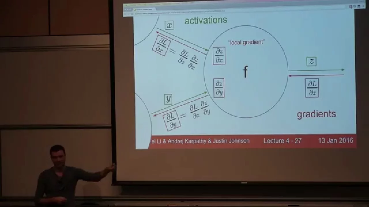
79:38
Lecture 4: Backpropagation and Neural Networks | Stanford CS231n 2016
@andrejkarpathy4906
322.7K views•2016-01-14

18:41
Neural Networks Explained: Math, Layers, and Learning Fundamentals
@3blue1brown
21.9M views•2017-10-05
Related Study Plans & Knowledge Roadmaps
Structured learning paths in Artificial Intelligence
artificial-intelligence
Aligning LLMs: DPO, TRL & Custom Datasets
01Foundations of Python & Machine Learning
02Transformers and Large Language Models (LLMs)
03Aligning LLMs: SFT and RLHF
+ 3 more learning modules
24h6 modules
Explore Roadmap
artificial-intelligence
Federated Learning: PyTorch, Flower & Privacy
01Python & Machine Learning Foundations
02Deep Learning Basics with PyTorch
03Introduction to Federated Learning
+ 2 more learning modules
35h5 modules
Explore Roadmap
artificial-intelligence
Securing LLMs: Guardrails AI & NeMo Gateway
01Introduction to LLMs, Python, and APIs
02Understanding LLM Vulnerabilities & Threats
03Defending LLMs with Guardrails AI
+ 2 more learning modules
15h5 modules
Explore Roadmap
artificial-intelligence
Building Recommenders: Two-Tower & Vector DBs
01Foundations of Python & Machine Learning Basics
02Introduction to Recommender Systems
03Deep Learning & Representation Learning
+ 3 more learning modules
75h6 modules
Explore Roadmap