




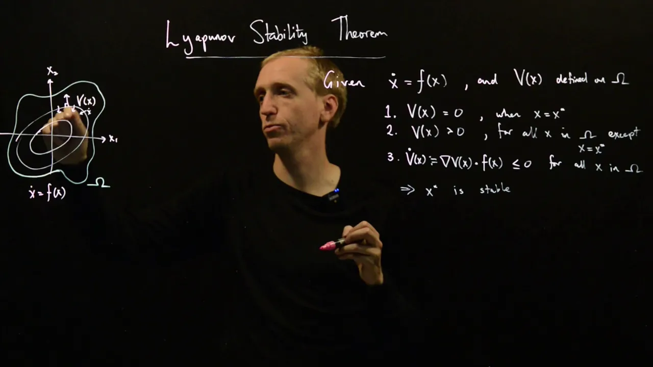
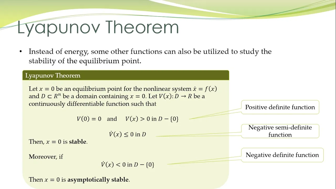


![[Tutorial] TF2202 Dinamika Sistem - Responsi Pra UTS 2024](https://i.ytimg.com/vi/xxJgHmJ0Ea4/maxresdefault.jpg)


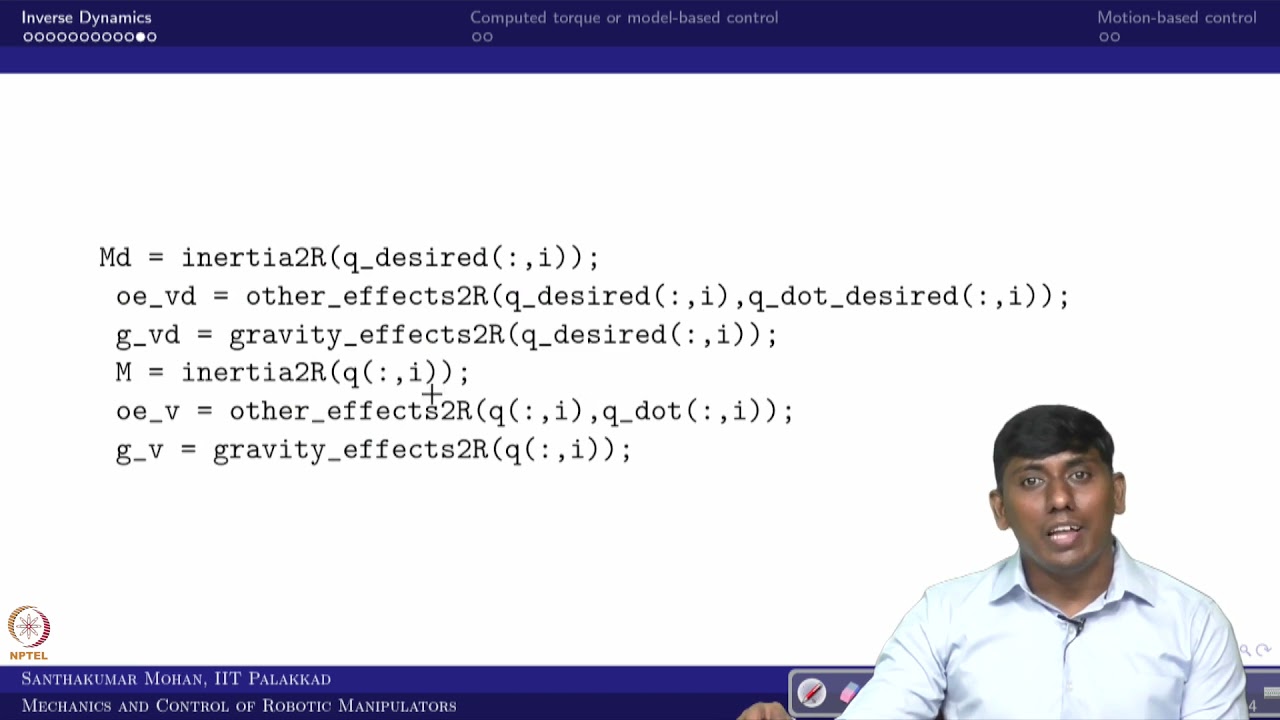


![[서울대학교 공과대학] 전기기기제어론 22. Vector control 1-2](https://i.ytimg.com/vi/3YmB_jaT5u8/maxresdefault.jpg)
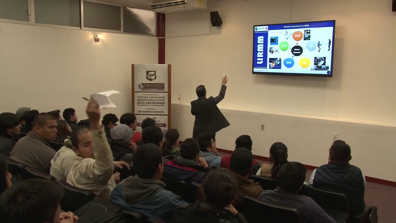


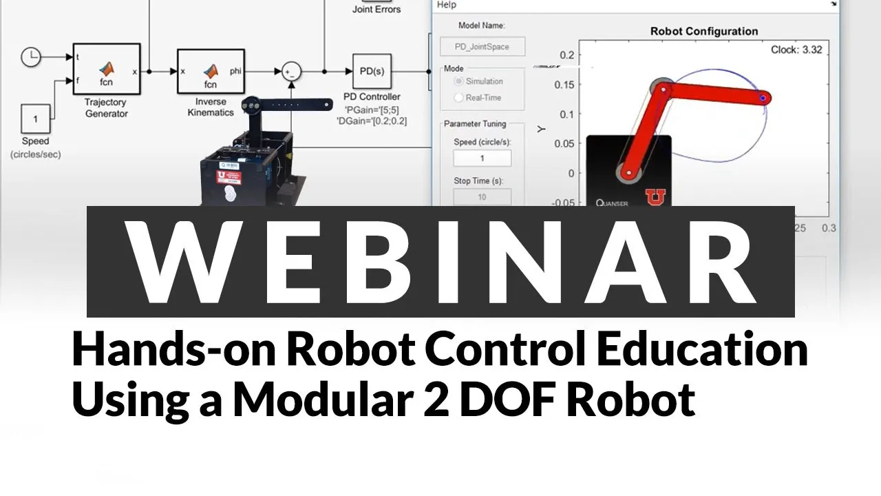


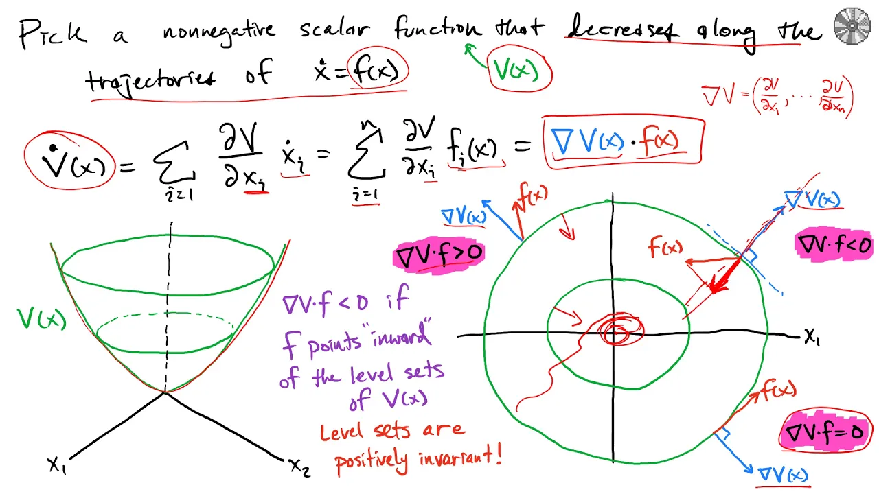
This lecture covers the theoretical foundations and practical implementation of PD (Proportional-Derivative) and PID (Proportional-Integral-Derivative) control strategies for robotic manipulators. The PD controller u = KP × e - KD × q̇ achieves global asymptotic stability for desired equilibrium states when gravitational effects are absent, using Lyapunov-based analysis with a candidate function combining kinetic energy and quadratic position error terms. When gravity is present, constant gravity compensation at the desired configuration (u = KP × e - KD × q̇ + G(qd)) ensures global asymptotic stability if the minimum eigenvalue of KP exceeds a bound α related to the gravity gradient norm. The lecture addresses practical implementation challenges including decentralized control with diagonal gain matrices, velocity estimation through numerical differentiation, and realization of non-proper transfer functions. PID control extends PD with an integral term to eliminate steady-state error from gravity mismatches, with stability conditions derived using the Routh-Hurwitz criterion. Saturated PID control prevents integral windup while maintaining robustness against modeling uncertainties.
Robotics 2: PD Control and Stability Analysis (Lecture 14b) | Prof. De Luca
Added:so let's start considering the first controller for the problem at hand consider our robot with its full dynamics the inertial terms the correlations and typical turn the gravity terms and our goal is to regulate namely to obtain a synthetic stabilization of a desired equilibrium state in the closed-loop system the equilibrium state has indeed zero velocity and a desired configuration to D now if you would like to design a control that is able to achieve this task and we consider for for the moments that the desired controller is of the form u equal K P times T V minus Q minus KD q dot this is a what is called classical PD control with respect to the position error so proportional terms with respect to the joint position error and the proportional terms with a gain KD with respect to the velocity ever so the derivative of the position error having in mind that QD is a constant if we take the derivative of the error QD minus Q we will have QD dot which is zero minus Q dot and so you see that the second term can be written as a derivative term with respect to the position error mainly the velocity now indeed consuming the desired q QD may come from kinematic inversion of a desired pose of the end effector but this is a different story so at this stage we have a desired configuration in this control law we make an assumption you will see that this is necessary also that to gain matrices are both positive definite and without loss of generality we consider them cement now the first thing that we would consider is whether this controller satisfies the condition for obtaining an equilibrium in the closed loop that is at the at the desired configuration in fact we see that if we are in the desired state so if Q is equal to P desired and Q dot is equal to 0 and you would like to be in this particular state so the acceleration without Dodge should be 0 plugging this controller in the above robot model would even on the left hand side 0 for the inertial term 0 for the velocity term and a gravity term which is equal to G of Q desired while on the right hand side nothing would happen so you would have the possibility of regulating eventually only configuration to desire which 0 the gravity term so this is a quite restrictive condition and so we will put ourselves for studying the behavior of this simple controller actually you see that you can imagine of in terms of dynamics in the condition where G of Q is identically zero in fact we have a theorem that we were going to prove now it says that in the absence of gravity so when G of Q is identically zero not just at some configuration that just vanishes in the model so the motion occurs at constant potential energy the desired reverse state qd0 so with zero velocity is a globally asymptotically stable equilibrium under the given PD joint control so before entering into the proof it is worth mentioning that despite the highly coupled and nonlinear dynamics of the system a linear control law like PD control is able to achieve quite important results so how do we proceed we will make use indeed alpha the machinery that we have developed in the first part of this lecture namely the upon of condition for stability and possibly asymptotic stability and eventually the use of the solid field so we defined the error as QD minus Q and we introduced the advanced candidate we have already seen that energy argument can be used very often left done this for the simple passive pending system but now we have to take into account that we are introducing also a controller so this the upon of candidate which is quite natural and see more of this type later on consists of the first part which is the kinetic energy of the system there is no potential energy because potential energy plays no role it's constant in this in this context because G of Q is equal to zero so this constant may be said to be off very well but because we are investigating a generic configuration to D as potential globally asymptotically stable ability we have to include in this function something that vanishes when we are at the desired configuration and otherwise is always positive in much the same way as the kinetic energy vanishes when we are at rest and all otherwise is always possible so we introduce the second term which is again in quadratic KP is the matrix that we are using in the control law so this does show shows that KP can be taken symmetric without loss of generality in fact it appears inside four and E is the position error and KP is positive definite so this second term by itself is always positive unless the error in the drum space is still so we have a good candidate function which is always positive except where you like to be so in the desired close to equilibrium States here we've got you and without the posse so let's consider now the time delivery of this function and we will evaluate this time derivative along the trajectory of our robotic system so the trajectory the evolution that satisfied the closed-loop dynamic equation of the system remember that gene of Q is equal to 0 so this closed-loop dynamic equation will be M times 2 double dot so the inertia times the acceleration plus the color sensor typical term equal the PD control so let's do the derivation first we have the quadratic term we have done this computation of ready once when we looked at the derivative of the total energy of the system and we discovered a nice property which we will use right now so the first term produces in fact two contribution in fact three but two are just the same so when we take the derivative of the velocity on the left side and on the right side we get the same scalar so twice is a scalar eliminates the factor 1 over 2 so the first term is Q dot transpose mu double dot and then we have the another term which is the derivative in which we take the difference there even if only of the inertia matrix so we have 1/2 to dot transpose and don't q dot for the second term we have exactly the same symmetry so there will be twice the same scalar contribution with the factor 1 over 2 and K P is constant so the only remaining term is 1 in which we take the derivative with respect to time of one of the three and our stirrups for instant the second one so the derivative of 5 e dot because you desire this constant is simply minus u dot so the last term is minus a transpose K P Q dot now this is just the time derivative of the function we should evaluate this function along the trajectory so we substitute the model please note that I dropped dependence in the inertial term and in the derivative of the inertial term and so on just for compactness so we have a term which is MQ double dot and 2 double dot appears also in the model so we are not substituting yet the control law so the only other term the bother are the correlation typical term and we know that we can always factorize this as the product of our nice matrix as a function of Q and Q dot and Q dot because those velocities are our quadrant so we substituted mg double dot u minus s Q dot we factor out the 2 dot transpose in front of these two terms and we leave the other time untouched others are by the principle of conservation of energy we know that this term this quadratic terms in the velocity so 1/2 and dot minus s as a matrix but Radek form in the velocities in fact a m dot minus 2's this is what we proved that this is a just a factor one house in front of this when put into the quadratic form in velocity vanishes and this is has nothing to do with the fact that and dog minus 2's maybe skew symmetric this is a property that holds no matter which factorization you are using in fact our control law does not use at all terms related to the model and in particular to the color sensitive little turn so this analysis is independent of what he are going to implement so this two terms in fact vanishes and this is a big advantages because otherwise we would not know what is the main sign of disturbs so the next step is replacing the controller at the place of the U so u is KP times e minus k DQ dot so the two dot transposing before the parenthesis give rise to the first two terms in this expression while the last term is being untouched remember that each of these terms are scanners so they are equal to their transpose in addition KP is possibly definite and symmetric so KP transpose is equal to KP so the first and third terms are in fact one opposite to the others wants to transpose one of the two and what is left is minus P dot transpose KD Q dot which by the choice of having second gain matrix the KD derivative term positive definite leads to the fact that this expression is non positive so it's negative one without this difference of zero and is 0-1 without this equal to zero again you see that the reason why we have chosen without loss of generality also KD as a symmetric one is because it appears then in the analysis in a quadratic form so only the symmetric part really matters so up to now we have fact proved only stability so if we apply the first criterion says we have found a lack of candidate the it's derivative is less or equal than zero then the equilibrium the one states that zeroes the Lyapunov candidate is stable but in fact this is not pieces of our theorem in fact there's still something to do in particular by the use of massage theory so noting that the dot is equal to 0 if and only if the velocity is the Sun so we have to find the largest invariant set of states that is contained in the set of states that 0 the derivative of the Japanese candy and this set of states is made by all possible configuration not just to be having Associated identically 0 velocity now in this set of state we have to find the larger set which is invariant it means that if we start from that set we remain all the time in that set so it should be a set where velocity is always seen otherwise it's not a subset of those states that zero the derivative of the yamuna canada ok so we have to find the largest possible imbalance set with this characteristics so when two dot is equal to zero we substitute this into the equation of the closed loop dynamics so the coral sensitivity vanish also the derivative turn in the control of vanish so we are left with the simple dynamics M of Q double dot equal KP times the position error since the inertia matrix is invertible we can isolate always duration and rewrite the formula like written on the right inside acceleration is an invertible some non singular matrix times the position error which means that if and only if the position error is zero then the acceleration will also be Z and so we will stay within the set of state at zero the velocity so this is an invariant sets definition on the other hand if the error in position is different from zero we will have a dip an acceleration different from zero so in the next instant of time we will move out of the zero velocity state which means that if the error is different from the position error is different Europe we are not in the condition of imbalance of an imbalance el sol La Salle tells us that the only possibility for of convergence is to the set of state that has also zero position error and therefore the conclusion integral as the corollary says the unique stay and she's invariant in the set of state that zeros the derivative of the yamuna candidate so have we got possible is the one with Q equal to desired which means in position zero as well and this concludes the proof is very elegant proof is also paradigmatic in the sense that later on you will see more and more complex we have one of candidate and analysis but essentially the principle remains the same now a note there were no particular specification on the structure of the two KP and KD so they should be positive definite they can be symmetric so there's no occlusion to the fact that we can choose them fully diagonal if we choose a diagonal gain matrix K P n diagonal gain matrix K D respectively the one that multiplies the position error and the one that multiplies the velocity we obtain what is called the decentralized linear control for each control command for each joint so you are I will be just KPI times the error in position at that joint minus KD I the velocity of that joint so it's purely local to the chart there's no need of having any information coming from the rest of the manipulator this is a also an important consideration from the point of view of software and if you are doing some say maker activity so you build some kind of robot by yourself for instance using Lego mind storm or something like that this would also help in removing connection with one run to the other so each joint received just the command of desired configuration of the truth reach and all the rest is being done locally in fact we can also give a very nice mechanically Division two this PD control and this is particularly true if we assume that KT and KB are diagonal matrix although although something similar to be constructive even for KPMG which I still see magic and positive so imagine that you have a planner robot with three rival joint and the desired configuration is the one as shown in orange now this plane is the horizontal plane because we are assumed so far that gravity term is not present so potential energy should because now we associate to each value of the two game uses either a stiffness of the spring so a spring stiffness API adjoint I or a viscous damping elements with damping coefficient K di and we do accept to the following suppose that we are in our generic configuration the current configuration is the one in green and this may be also the initial configuration at zero at zero velocity now in order to obtain the desired configuration we place some reference stick in the sense mounted at the base of each sling and connect this reference stick to the associative link in a decentralized way as I said through the spring of stiffness KP and damping element with viscosity KD pay attention that the way in which we are assigning this reference is relative to the previous tree so you can see that for the first link the red bother the orange bar is exactly in the orientation of the first link of the desired configuration now the second being in the desired configuration should make an angle of ninety degree actually 90 degree positive because is counter there sorry negative because it's counted there clockwise with respect to the first link so the second reference bar is placed at minus 90 degree with respect to the first time at the end of the first link or at the base of the secondly and we connect then your spring and damper to the second a similarly the third link should make I will say 45 degrees or maybe 60 degrees the first time I was thirty positive with respect to the secondly so we mount in that with that angle the last stick which is the reference we just assign directions third joint and we connect again KP 3 and KD 3 games which are mechanically a spring such sickness hibiscus this touch coefficient K VI so if we keep everything we hold this device for a moment and then we leave it so we start at time zero with the evolution the motion of this mechanical system subject to springs and dampers will be the motion of our robot where all this machinery this mechanical object are not there but we have a software commanded PD controller but revolution will be same and you can imagine that the robot will start moving accelerating and then oscillating and then damping away its velocity until it stops and the only position where this system can stop for sure is the desired configuration to do so this is a nice mechanical interpretation you could also build a device that does this at home just with mechanical objects of Springs and both the stores and with this Lego or mechana like construction you can prove that everything works as we have now this next slide shows what happened why do you need to use LaSalle's theorem and you cannot we are not able at least there's no such candidate known to prove directly asymptotic stability without resorting to yattaman - la sala theorem so this is a qualitative behavior of the optimal candidate at time zero we supposedly start at rest so kinetic energy is equal to zero so the remaining term in the candidate is just the quadratic term in terms of the positional so we start with a value which is known because we know where we are we know where we would like to be KP is a game in our controller so it's something that we have chosen so we know for sure that we start from a known value B at time zero is zero which is which is shown on on the on the graph it's the first now by the way forget to say that these second terms with this mechanically degradation is exactly the potential energy associated to those set of Springs that we mounted on there on the physical system so we can use this mechanical interpretation by saying that the system has in fact that the candidate function is in fact the sum of our kinetic energy of the real system and of the potential energy of the springs of this vehicle system in fact this potential energy is the potential and just to see the two our control law there are no Springs at all but this can this interpretation can be given by this example I show now at time zero the velocity is zero so V dot which is minus 2 dot transpose K in D times Q dot is also zero so the tangent of the function V of the evolution of the function field over time so we don't in fact because the x-axis is represented by time is horizontal but as soon as since we are not in the desired configuration because the error is different from zero otherwise the function V would start from zero and we are already where we should be so the acceleration will be different from zero so the system will move so we will get some velocity and for sure the value of the content of the the apana function will decrease because V dot will be negative if you don't is different from zero no matter if P dot is positive or negative you see that this analysis is made on a single scalar function without making reference at all of what is the type of robot how many joint has the robot what type of joints are it has the only condition that we have said so far is that gravity plays no role so G of Q is identically 0 otherwise this consideration are fully general so the level of function will start decreasing and it will never go over the value of V of 0 because in order to do that it should become should have a for some instant of time a positive time variable and this is never decays so it decreases it start decreases faster slower this depends on many aspect but suppose that at some time we have a flat plateau where without is equal to and this can be repeated several times now without can be 0 only if the velocity stops sources the velocity is equal to zero which means all the nos ''tis of all joints are simultaneously so this happens during the transient because you have a kind of motion inertia now the easiest way of thinking about that is considering a single horizontal me and which is initially at rest and suppose that you want to do a a slew of 90 degrees so you set plus 90 as your reference and then you let this link move now the link will approach the desired angular position but typically would overshoot it and will start oscillating and then then pin out its velocity around the desired configuration until it reaches the final value of 90 degrees now every time the system inverse motions of the linkage where the motion is scaleable in this case there is only one singular one single value of velocities the velocity will go to zero from positive to negative and this is exactly where the Nahanni function will have a single instant in which the tangent to the time profile will be horizontal but indeed that could not be a finite interval in which this remains zero because otherwise we would have also acceleration zero during that interval and this by the analysis that we have made can happen only when we have reached final destination so when he becomes zero together with the velocity so this when this happens not only the derivative will be 0 for a finite interval but it will be zero forever destination so this is a very interesting consideration the rate of change of decrease of V depends on the actual robot on the actual gains on the initial states on the initial configuration how far we are from the destination and so on but this general behavior is rather common that could be also basis in which there is no instant in which all the joint velocities are 0 [Music] at the same time so you will only see a decrease it could be slow but asymptotically the menu will go to 0 as shown in this picture now few other comments on this PD controller remember that gravity is not there so we move after these comments the presence of gravity so first of all indeed we have said that KPN TV can be diagonal or in any case should be positive definite if they are diagonal is positive definite occurs if and only if all the elements of the diagonal are positive but in general you could choose also KPN Katie but even in the simple case when you choose diagonal Killian PD so if the robot has for instance six joints then you have choose six games for the proportional terms and six games for the deliberately the element of the diagonal of this 6x6 matrix now this should choosing the right games before beside being possible of course there are many possible choices and it's the choice that you make will affect the tie the nature and the duration of the transom and also the practical section time in the sense how long will it take until you are close to the desired configuration close enough indeed since we cannot prove exponential stability but only asymptotic stability we have no clues on how long will be the strength so you could start doing test trials and tune the game matrices so that the behavior is optimal but one set of value may be good for excuse for a given robot for a specific motion for another motion another set may be superior so having an optimal behavior over all possible motion and all the whole work space for a given robot is a very hard task sometimes the choice of a full gain means it is so not time to know helps in defining the value of KP KD which works reasonably well at least getting closer to the destination why because at that time we can use the linear approximation of the model so the closed-loop system in which KP and K V appeared and used the degree of freedom to assign to the linearized approximate model which holds as long as you're closer to the destination so small velocity and Q deep - current Q small enough at was sandy eigenvalue to the closed loop system so on the linear system we know that for instance assigning real eigen value with a void oscillation overshooting and something like that if we move far away to the left of the complex plane the eigen value we know that this is has seceded to a rapid increase lead with a larger value of the control laws or with more effort and so on and so on so this is the reason why full KP NPV may be useful exactly for tuning them taking into account what happens close to the destination of course the initial transit would maybe not the best one that you can achieve and there's a large variability so to make long story short the tuning is very hard in this context the tuning of the games the second comment is we neglected any type of fresh let's consider just for a moment the presence of viscous friction at the joint so an effect which is a subtraction of energy from the applied controller remember that dissipative term happens to appear in the dynamic father on the right hand side of the Euler equation exactly where also the control is active so in that case viscous finished viscous friction term would be of the form minus F v2 dot where FV is a diagonal matrix and on the diagonal you see the viscous friction coefficient for each joint now this term looks very similar in fact act very similarly to the third minus KDT Dalton the control law in principle if your guarantee that you have in us enough viscous friction in your system you can also achieve global asymptotic stabilization of any configuration without the derivative term in your controller because the damping is made by the viscous term which is present in the system indeed if the viscous term is small you cannot rely in a very fast transient so dissipation of energy fast enough for your name and this is why you introduce in any case terms the other points which concludes this set of comments is that when you have a full BD you need a measurement of position John position which is obtained by encoder this is the standard solution you may also have system you shall analog sensor of position like the solvers or potentiometers but this is more and more obsolete but you don't have typically a tachometer for measuring the velocity so you need to make some kind of numerical derivative of the position measurement in order to have an estimate of the current velocity to be used in the controller and this can be done in several ways so let's look at the problem from a continuous or a discrete-time quantity so suppose that this is the starting control over so your T 2 T because I would like to see what happens when I'm sank in this controller or when I'm implementing directly a digital controller which is updated at every sampling time so U of T is KP times the error but that instant plus KD times the derivative of the error at that instant where the derivative of the error is nothing else and - to go this is the euler design this is the control over which we improve an asymptotic stability now if we since this is a combination of signals and linear combination of signal in fact we can use la Pan's Laplace transform in order to represent this is the Laplace domain I hope you're familiar with this notation if not you replace every signal which is transform the domain s complex the mean s so e of T becomes s and every time you have a derivative of a signal the transform of this signal differentiable signal is s times the Laplace transform of the original one in the same way if you have an integral term of your signal you will have as a transform a factor 1 over s the transform of the original signal so in our case when we move to Laplace we have the transform of the U of time so you have s equal KP the transform over time and then plus KD to transform of the derivative of time so this is s times G of s so we can see that seen from an input point of view if we take the error as as the input of our control the position error as the input of our controller and we generate U which is a PD action of this signal so without an information about the velocity effect the transfer function of the controller will be KP plus KD s so there is a juster function without any denominator so this would be a numerator only so this this transfer function from s to every command you output from the controller is a non real install some so this means that if you don't have a measurement of 2 dot which means of dot you cannot realize this except so in general when you have a non realizable transfer function so one function as a ratio of polynomials with the polynomial denominator having degree larger than polynomial denominator so in this case the numerator has to be one that there are neither has to be 0 because is not there is this one in fuchsia then in order to obtain a realizable implementation you take the derivative term so the terms KD times s and you filter it at the certain bank so you add the pole with a constant time tau a small constant time which means that up to the frequency 1 over tau you're taking the correct derivative beyond that when this pole intervenes in the frequency response of the system you're not really doing that doing the dirty believe in yourself okay now if you look at this transfer function now and you come on so you will have 1 plus tau s in the mini a terse or polynomial is degree 1 in the numerator you will have KP plus KP tau s plus T yes so again the numerator will be a polynomial degree 1 so you have recovered Casali in essence this is a Robert transfer function in fact it's the sum of our constant gain plus a strictly proper transfer function so this is the way in which you in kinetics if you had an analog system then you would implement this type of transfer function one that is proper and then realize and this means that in practice you're not taking derivative of all frequency component of your signal of your ever signal but your limits for even bandwidth the very muddy Bank so you're doing an approximation now what if you're implementing this in discrete-time so there are many ways to get there I will use the so-called theta transform which is another transformation in the complex domain which is associated to a sequence of samples in general this is the transform and you can have mapping between the Laplace complex domain and the Z complex domain so the two complex plane can be met one to each other depending on how you implement derivation and segregation for instance if you use the backward differentiation rule on the samples we should acquire and generate every TC second for instance every TC equal one millisecond using this dagger sampling time then the s is substituted by this one minus e to the minus one times TC now I will be not detailed this because either you know what I'm talking about or it's kind of difficult to explain in short but essentially each factor is e to the minus one is equivalent to a delay of one step so if you take a signal at this is the instance T or T of K and you take the same signal in the transform domain pre multiplied by Z to the minus one you're using the value delayed by one step so you're using the time TK the value at time TK minus one so this is the digital version of original pretty not realizable transfer function you will see that in the digital domain since you're computing things based on the current and on the previous component or samples this will turn out to be realizable as well in much the same way you can do the transformation on the transfer function of the bandwidth-limited pd action so you replace even in the same context you replace two each s that you encountered in the transfer function the expression 1 minus C minus 1 divided by TC and now you can go back to the sequence of samples and you recognize now that both digital controllers the discrete-time implementation of this PD action are realized so they don't use future sample in order to compute the current one they can only use the current samples or samples from previous instant so if you go back to this transformation you elaborate things the first expression says that the current command torque of man that you're sending to your actuators is KP times the error of that instance of the position a terrific instance plus KT the difference between the current ever and ever at the previous sampling time divided by the sample time interval ok this is our what you have would have done probably right from the start looking back at the time domain expression of your PD when he implemented in dot you implemented as just the difference between the current value the previous value and the duration of the time interval of same but here you can see also a slight variation if you want to implement this by giving some limited bandwidth to the deviation which means also that you're filtering any noise at high frequency associated to this derivation then the resulting district and presentation is slightly different in fact you can recognize the same proportion action this is an instantaneous actions of KPFK the last term's is similar to the discrete backward differentiation so you're taking the two-sample a cave subtract a K minus one and you divided by the sampling interval but you add to this also the small time constant tau and typical tau is 1/10 of T see this is almost the same what is new is that you have an extra term which is based on the last control sample that you had computed in the previous Sandinista so this type term tau over tau plus TC times U K minus 1 this gives some continuty some smoothness in the sense to your results ok this was a few words on the implementation in the digital context of a PD controller now let's move to the next subject so let's say okay so far we had no gravity so the mother was M of 2 times 2 double dot plus C of Q dot equal the command what if we have read like him I would say most of the cases we have seen where gravity can be neglected or is absent so signaling for planar motion on a horizontal plane in the far space where gravity has little or no role but of course there are other problems there and so on so what if we have a certain manner it's the standard situation which of Q is present we have already seen that the PD controller is not enough because it does not guarantee that the desired configuration is an equilibrium there could be another equilibrium in fact the roster system would not the design one so the simplest way to handle the presence of gravity is to cancel so this is a really a nonlinear action will control why because if your controller is the PD action as before so KP times to be minus Q minus Q times Q dot and you're adding these terms in the controller so your computing based on the model information the gravity vector and using also the current measurement of the joint angles G of Q so you will have this on the right hand side on the left hand side you had now also G of Q so these two terms are equal and cancel each other so if you are applying this type of law you end up with the system which is exactly as before so without gravity in the dynamics and just with controller so there is no need of any analysis or proof using the same argument you know that this type of controller globally asymptotically stabilized the desired state Q equal to D and you got people 0 under the assumption that KP and K we are possibly dead okay it's nonlinear because the evaluation of G of Q is not only the variation of further and it contains not only sums and products like in the PV part of this controller but in general trigonometric evaluation so you have to store to evaluate sine and cosine of different combination of T so it's slightly more complex and also the analysis in this case nonlinear controller you have still a nonlinear problem so you cannot use linear techniques like for placement or eigen values and so on where to do with non-linearity as such and this is why we developed all introduced all make reference to the vehicon of analysis which works both for the [Music] the main difference is now that if you cancel gladly you have to know at least those it turns particular you have to identify the dynamic attrition which are present in the gravity term of your table and this may not always be the case for instance if you grasped in an object online you don't know the object's weight and this will change many parts of the model but in particular the one the gravity turns actually needs to implement this controller so this is no longer and non model-based control action we don't have to know much of the model but at least the gravity term should be no so what happens if you have just an estimate an approximate estimate let's call this approximate estimate G hat instead of the corporate CUSO the model has a G heads and so you are using this information in your controller the real system has a G of Q the real one and these are different they may be different for many reason for their structure but in particular they may have the same structure but the dynamic coefficient may be different in the two cases so one particular case is when jihad is vanishing so you're just applying PD controller then you know that you're not get the desired key D so whatever she had you're using an approximate one none of it a very good one instructor but with the wrong coefficient and so on you will end up with a steady-state final position which has an angle so you get to some configuration Q star which is different from 2d and depending on where you're starting from how far you are at the beginning and probably under dynamic characteristic even the inertia characteristic of this Q star may not be unique and so you can reach different steady-state situation all wrong with respect to the desire to design if however you increase KP enough without bringing it to infinity but there's a lower bound hippie that guarantees that this steady state configuration to start that you reach will be unique and the larger say keeping the closure will to start a bit to the side but the same bring it to zero this difference so having the desired equilibrium as the desired configuration as the equilibria in the closed room with this type of controller when G had is not the correct G occurs only when you drink now you can given a nice interpretation true to this results of having this steady-state error because when you're reaching the steady-state sorry you're in a configuration where the gravity term becomes constant and you can consider this as a disturbance acting on your system without this disturbance so without the presence of gravity you know that the PD would work so you would bring the system at steady state to zero error situation instead at steady state you have a constant disturbance because of this because of the presence of gravity and since the system control has no integral action before the position in the block diagram where this disturbing Tory actually is acting then you expect to have such type of it in the pieces are just a linear interpretation of what happens but it's pretty much a good one in fact you will have this steady state ever and you can reduce this theory study ever by increasing KP but only keep going with people infinity this will go to zero otherwise you need to entity to introduce some interaction and we will see now the next console also in the presence of gravity the first thing that you can do is cancel grams and the controller because of the the leaner one however you could do something sometimes more smart more simple to implement in particular the reason why without the gravity term in your PD you would not regulate your desired configuration is because at the destination if there is a gravity term if the gravity is acting in the final configuration you have to compensate for it so the idea here is why not modify the PD control that design the absence of gravity by ending a constant term which compensate gravity only at the station you add it from the beginning but this value is the value that we remain also at the end when the position error is going to zero the velocity has gone to zero so you will be left in the controller with the gravity compensating the asset at the destination so you would like to add a term which is G of QD to see this and then study if this works if the fact that this is the right command at destination does not imply so it's an equilibrium the possible system has the desired agreement does not mean that discipline is and stable and even that is global is affected unstable so depending on where you start he may end up you know you may get stuck in some intermediate consideration so we need an analysis of this and you will see that this analysis it is a bit more complex than the one of the people showed by itself in the absence of plan and we will use a structured property that we already mentioned when dealing with dynamics which is the following suppose that well the G of Q's of the vectors term emitted gravity contains the general trigonometric terms sometimes linear terms Q when we have prismatic joints but in any case there are structural properties that holds if you take this gravity vector and we take its gradient with respect to Q and you remember by the way that G itself was the gradient of the potential energy associated to gravity with respect to Q so the result will be a matrix a Hessian of the potential energy and this is the first expression so the structural properties that holds and we will not prove this but we use it the truth is that there is about an upper bound on the north of this minute so for any Q you can find over existing you can find a very alpha larger than zero that is greater than the norm of this matrix and this matrix as two equivalent way either the Hessian of the potential energy with respect to Till's on the second derivative or the gradient for the first derivative of the vector G irrespective of you a consequence of this using exactly this second expression is that if we take any two distant contribution it could be q1 and q2 for one and two as you see it's a different configuration of a robot and the user people or like it is written in the slide it could be the desired configuration QD and a generic other one and if you make the difference between the gravity vector in 2d and the gravity vector in this generic configuration killing than the norm of this say gravity error term can be bounded by the same alphabet its bounding the norm of the gradient of the gravity times the norm of the difference between the current configuration and the desired way and this is a very powerful inequality because on the left hand side you have terms depends on the model I mean directly on the right hand side Q minus GD does not that you have while the Alpha is a bound on some model terms and delivery of this model terms but indeed we can be very conservative so you don't need to know except in the value of the masses of the central gravity of this interlink all the dynamic parameters that happens to appear in the gravity so you have this inequality allows you to fill these from these dependents at least in the analysis the other note before we start with a controller and the proof is that those are matrices so the nor is intended as a matrix norm which is indeed by the induced by the standard original that we use for vectors so for instance in the expression in the yellow box all terms are vectors so these are vector norms and we can take for its a Euclidean norm so the P equal to standard mode so we when we consider instead norm of matrices induced by this norm on the vector and considering the mazes as operators or making vectors into vectors the Associated norm is the one shown here so the square root of the maximum eigen value of the matrix a transpose a now a transpose a is and if matrix is symmetric then we know that all these eigen values are real but some may be positive and some may be negative if you take 80 times a not only this is symmetric so all these eigen values are real but it's also semi positive definite so they are real and non-negative so you can order them from the lowest one to the largest one and you take the largest eigen value of a transpose a and you take the square root in a sense you're compensating the fact that you make the product of the matrix x transpose and this would be Bernard it and it's the norm in the sense that satisfy all the condition for a mathematical object to be an or and we often call this also for a matrix a a with capital you can also have this point since you have a list of five I can tell you take the smallest of this eigen values they will all be positive or zero so if you take the smallest eigen values that means if exposing a square root we will use the notation a small and and indeed this you would then capital and witches in order to make okay so this was the lawn but necessary premise let's see our controller pay attention this is a linear controller because there is no nonlinear operation on the measurement G the PD action is a linear feedback and the second term is a constant fit forward that you have computed once for all without any measurement Q so you can put this offline and then use it at runtime I will make also the preliminary assumption that KP and TD are positive definite and without loss that will this control works if we put this controller into the dynamic equation of the robot and we look at steady state conditions over to God is equal to 0 and Q double dot equal to 0 so we are not moving moving then we can see that Q equal to desire is an equilibrium ok with $2.00 policy so we need to show that this equation is asymptotically stable and this is what this theorem proves under an extra condition not only we have chosen can be positive definite but we should take the minimum eigen value of P transpose K P if P means otherwise the minimum element on the diagonal of K P larger strictly larger than the bound alpha on the norm of the gradient turn but if we choose this again it's a sufficient condition then the desired state Q equal to desire them to don't equal zero using the joint space PD control plus constantly gravity compensation actually so we are not cancer in gravity everywhere but just adding the term that compensated at the destination then the closed-loop system and this will globally asymptotically stable exactly the same result that you get without gravity with the simple TV or gravity with cancellation at every configuration of the now the proof first of all we have said that the QD 0 is an equilibrium state for the total but this current is that the control makes sense but the first thing that we have to deal if we want to have globality is that this is the only so the unique closed with the collision of the system so let's look at the equilibrium solution so when we have Q double dot is equal to 0 because this is from our states of the dog is also zero so what is left is um let's say on the left hand side of the Model G of Q only on the right hand side of the equation of the model we have the PD plus gravity compensation and destinations of the years k PP plus G of QD of course the derivative term is gone because the velocities here so if your rearrange things you bring one term to the other side you will see that we have this equation holding at any closer so maybe e equal J of Q minus J to be indeed if we put them there q equal QD the right hand side becomes 0 the error e becomes 0 and this horse this is in fact what we have commented before but we need to show that this is the only way which this identity can be satisfied in fact if the word another close to the Gribble which satisfy this so with a Q different from QB then we have the following chain of inequalities so we take the lord of the left-hand sides of the economic KP times e and this is larger than equal then the norm of e times the minimum possible value of KP let's say on the diagonal okay so we have the first inequality the second inequality is the one that is in the hypothesis of this KP minimum is strictly larger than alpha so we have at this term with the norm of e is strictly larger than our Thomas he which is QD minus Q or Q minus QD and buy the property justice alpha is a bounded turn on the reading of the gravity vector this is larger or equal than the norm of G of Q minus QD and if you look at this chain of inequality and you have a strict inequality at the center then you see that if Q is different from to desired and you should have still the balance of the two terms but on one side you have the norm of the left-hand side of the equality which is strictly larger than the norm of the other side and this is impossible in order to have the equality holy so this proves that the desired configuration in the third stage the closed loop to D 0 is the unique closer now consider that I am fond of candidate the level of candidate now it requires some explanation so the first of all we know this that the first part is exactly the same one that we used for coding PD in the absence of gravity so there's a virtual spring term which is the controller for turning the KP there's a kinetic energy and then we add also the potential energy because now the gravity is present we subtract this the potential energy at the desired configuration and we have also a term which is the product scalar product of the gravity vector at the destination times the error in position and this is a kind of a mix of term which appears to be coming out of the blue in fact it is not obvious that this is neither the fact that you have all the three last terms so you have a some kind of modification of potential energy is because you need to have a ally upon of candy that which is strictly positive outside the desired state so you need both of this term so let's see if this is a dysfunction that we have introduced simply as that is a candidate so if it is positive for any state except the desired one the desired equally nice work Q is equal to P desired so that everything on thank you dr. simple to see now in order to show that this is the case of that this is the right candidate and this is the most work that we have to do because otherwise the rest of the proof is really application of the same technique that we've seen before so we show that this function is convex both in Q dot and in the error in fact what matter is the error the difference between Couvillion and and Q which we would like to bring to zero if we write it in this form not so that it's convex so it's increasing and it's 0 only for equal 2.40 so when we are in the desired configuration we have to zero velocity then this candidate is a correct candidate so in order to show this we take the derivative of V with respect to Q dot and with respect to the position error if we take the derivative with respect to Q dot Q dot appears in the function only in the kinetic energy so this would give remember V is a scalar so when we take the derivative with respect to a vector in this case Q dot we get a row vector so we need to in order to get a color so if we do this we think the derivative we would get twice the same quantity so we can remove the factor one half and have Q dot transpose times and when we transpose this we get M times Q dots remembering that the matrix the inertia matrix is symmetric so and this shows that this derivative is equal to zero so we have a minimum or a maximum if and only if the velocity is zero because M of Q is a positive definite now in order to see if in this direction we have a minimum or a maximum we should look at the second derivative and evaluate this where we have zero the necessary condition for stationary points and at first if we take the second derivative with respect to Q dot then we ends up with M of Q this is positive definite so this is typically associated to a minimum what about the other direction so we see that we need to have two dot equals zero in order to zero the function so we take the derivative with respect to God ever when Q dot physicals so we neglect the presence of kinetic energy missiles so in the remaining term we have the first term is quadratic in the error so the derivative and then transposition just like before in order to get a column vector is equal to kV B then we have the derivative of the potential energy U with respect to e but remember that E is QD minus Q so taking the derivative apply a chain rule so the derivative of U with respect to Q is just the derivative of U with respect to either sign - because we have the chain rule the derivative of V with respect to Q is - the ident so the second term is minus u over the Q and then we have to transpose it so you have that term then we have - you came D U of Q D and this is a constant so it's derivative is zero and finally the linear terms in the ever so when we take the derivative with respect to B and transpose this we get exactly G of PD now remember that the gravity term is nothing else than the gradient of the potential energy so the second term is in fact G of T so we are left with the condition that the derivative with respect to B second set of variables of the error method is to place the cue with the error is KP e plus J of in D - JT and in order to have a stationary point we have to zero this term but this is nothing else than the equilibrium that we studied before and we know that this happens to be zero if and only if Q is equal to QD and the fact that this stationary point is a minimum is shown by the second derivative still evaluated at 2.40 with respect to the error so V squared B over in square so if we take the derivative of the previous expression we have again just KP then we have a G of Q we take the derivative with respect to e and not of Q so we have to change again the sign so we have a plus second derivative of U with respect to Q Square and since the norm of KP which is KP maximum so with the lambda max is greater or equal than KP with the minimum and this KP the minimum is larger than alpha which dominates the norm of the second term so the norm of B squared u over the Q squared then this shows that this quantity will certainly be positive and therefore this is a meaning so the function increases and has a single minimum as we have seen in the common configuration in the states in the desire states Q for Q T and equal 0 and this is what our conclusion is now shown on the slide so at this point we have to look at the time derivative of this candidate so the function is a candidate so it's a good point to start with and we take the derivative and now I will be more speedy because the first two term they have derivative is exactly the same as we have found before so Q dot transpose times the terms in the bracket minus C transpose K PQ dot now the next terms is the time derivative of U so again chain rule the time derivative of U with respect to U and then of Q with respect to time which gives us Q dot and finally we have a constant term which vanishes in the delegation but then he transpose G of Q T again we take the time derivative of e dot which is minus Q dot transpose times G of T we substitute the model because we have to evaluate V dot along the trajectory of the closed loop system so first we not replacing the control also 2m u double dot we replace the terms U and then we bring everything on the right-hand side so minus s times G got minus G and then there's another term that was already present with m dot in the bracket and on the last two terms we take that this is a scalar do over the few times to God so it's equal to its transpose so we have Q dot transpose times du the Q transpose which is nothing else than the gravity terms so we have a subtraction of G minus G G of Q minus Q DC I pre multiplied by Q dot transpose now we use again property together m dot minus 2's or what is equivalent 1/2 and dot minus s vanishes when being the matrix in the quadratic form with the same velocity outside do not transpose M 2 dot so this term is gone and then we replace the U with a controller which is KP e minus KD q dot and then plus J g of cuba's are all these terms are pre multiplied by Q dot transpose so you see that we have generated an extra term from the first bracket which is P dot transpose G of QD minus G of Q and the rest remains the same now this two term cancel because KP is somatic and one is the transpose of the other with the opposite sign and similarly this two terms also cancel so the whole introduction of extra terms in them yeah moon of Canada was meant to arrive at this cancellation because otherwise we would not know the sign of this term so this long story reduces in the fact that the time derivative of this we have enough candidate is exactly the same as in the case of no gravity so minus Q dot transpose KD to God with KD being positive and this one feels less or equal than 0 so let's see what LaSalle tells us because I've talked to now we have just proven stability so when we thought is zero if and only if the velocity or velocity are zero so let's look at the dynamics under this condition in the closed loop so the color is acceptable term vanishes so we have M of Q double dot plus G equal the controller where Q dot is now Z so it's just KP plus G of Q desired the constant compensation at the desired configuration so we can isolate the acceleration as well now the acceleration is carries over more terms than in the case of no gravity indeed but still we have we can isolate acceleration because the made inertia matrix is non-singular so we have M to the minus 1 times K P plus G or QD and then we have brought the gravity at the current configuration on the other side and now the acceleration will be zero if and only if the term in parentheses multiplying M to the minus 1 which is not secure is zero but this is zero if and only if Q is equal to Q desire so when the error is zero so the acceleration will be zero only if also the position error is zero and the South theorem says that we will converge to this unique a state which is the maximum variance set contained in the set of states which zeros the derivative of the Lyapunov candidate and so the result what this is the theorem follows so let's see an except now we do the most simple example that I could think of but it has also some peculiarities so I'm considering now as a pendulum so a single leap robot under gravity but now the robot this link is actually salt qualifies as a robot I see here you see again model so there's an this is a model distributed mass so we have an inertia around the center of mass moves to the joint axis so we will have the inertia let's say EC plus MV square and this becomes the inner shine I which multiplies the acceleration till double dot in the model on that in the equation below the picture and then we have plus mg 0 D times sine of theta which is the gravity term equal the torque that we applied to the controller now suppose that we can start from any point typically we start from the floor with zero velocity so T variable 0 and we would like to do a swing up so to bring the this single link robot in the upward equilibrium so the three DS are equal PI now in that configuration as we have already seen gravity vanishes like in the lower equilibrium so if we apply PD control plus gravity compensation in fact we are only applied PD control and the controller will be KP times u Lisa T the desired case so pi minus the current theta minus KD the joint velocity theta dot it would be plus G off to the desired but this is steel so this is a PD working under gravity because at the destination the gravity term vanishes but still we have to overcome gravity during the transient so the theorem says that even in this case we need to have a proportional gain KP which is larger than the Alpha that dominates the gravity gradient now in this case everything is scalar so everything is very simple so if we look at the grade the gravity term mg 0 D times sine of theta we can bound this since M is positive G 0 is positive and D is positive we can eliminate the sign and have an upper bound for this so alpha in this case is simply taken as mg 0 D so the theorem says that if our PD controller even without the gravity compensation term because this constant term is 0 at the destination for this particular case the proportional gain should be larger than alpha and the derivative gain should be positive in any case so if we look at the eye upon of candy that we have seen in general and we applied it this simple case and we look just at the section no no the Lyapunov candidate in this simple case is a function of only two variables theta and theta dot now so we show a plot of the level of candidates on a two-dimensional plane with a third dimension used for the values of V but this is not important it just can cross the the plane at at the value theta dot equals 0 because if theta dot is different from 0 the kinetic energy to be pleased so we just look at the worst case what is the values of what are the values of V of theta for theta dot equal zero and you can see that if you choose again and therefore the same game is being used also in the labyrinth candy which is smaller than alpha in particular is the half of alpha the first plot on the left hand side shows that you have stationary point one at PI so 3.40 but also two other values which are before and after the upwards equilibrium so on the left and on the side and these are relief minima while the other is a local maximum so this will be unstable innocence so if you let a ball roll if you start at rest on the upward equilibrium you will stay there but as soon as you give a perturbation your controller is not able to assist out you can stabilize the desired configuration so you will fall either on the left or on the side or on okay if you increase KP and you bring it exactly to the value of alpha should be strictly larger okay you see that the profile of the yakonov candidate in this section for theta dot equal zero will will be positive but again you have some kind of fun they receive your flatness as soon as you increase beyond the alpha value so in particular last plot is for KP five times alpha you will see that we have a single isolated minimum and to the desired equal to five so you only our condition will be sufficient but in this case by a local analysis approximation we can say that in order to guarantee not only can't be larger than alpha guarantees convergence and asymptotic stability but it's also necessary otherwise we could stuck in a different configuration so this was the analysis made on the equation and using the information from them the apple of candidate let's do some numerical simulation let's put some numbers so for instance we have we need only two dynamic coefficient I the inertia of the link around the joint axis and we take this value about one 0.93 it is coming from some assumption in the structure of the ligand and the second number that we need is the product of the mass times the distance of the center of mass from the joint axis time the acceleration 9.81 and put some number you get 19 point 62 you see you we don't need to specify more we don't need to know if the distance is longer and the mass is shorter vice versa is the whole project that matters so this will be also alpha the minimum possible alpha now if you don't know the mass or the center of mass but you know the link length then you can over bound this I mean if you assume that the mass here more or less it could be around five kilogram you say well it's not larger than ten kilograms then you double this number if you don't know if you have a uniform distribution of mass in the link so you cannot guess that the center of mass is that the health point of the link but certainly is on the link so you can over bounded by the link length which is a kinetic parameter and so you have an over a conservative value of alpha which is in increase which means that if you take a larger KP which dominates this conservative alpha your guarantee that everything will work so this is the way in which the reasoning which is behind this type of methodology now suppose that again you would like to do this simulation is a swing out from rest in the low lower equilibrium configuration so the link is downwards to the upwards configuration under 80 degrees so five where the gravity is zero so suppose that we choose now the PD game so we don't need to compensate the concept the gravity at destination because this is do we choose K P 36 and KD equal 12 so the P game satisfy the sufficient condition 36 is larger than alpha which is nineteen point 62 and this is the evolution from the position that goes from 0 to 180 as you can see in about 5 seconds even less getting closer the velocity so the theta dots that start from zero at rest hazard quite a large P of this is degrees per second on pages per second so if this is self about 2 pi per second and then goes quite amusing down to zero and the error that starts with 180 degrees and then goes to zero and finally the control effort you can see that there's a large initial torque about 100 millimetres forum link which is about five kilograms so this is a huge torque in a sense which is needed only for a few instant of time less than 0.2 second I'll say and then the torque goes down and add the equilibrium it is zero because we don't need tort to stay destination where the gravity is equal to Z so once the P term has gone to zero there's nothing else less so this simulation shows that things worse now suppose that we reduce the gains in particular we'll use the KP gains below the value of alpha now we have shown that by linear approximation this minimum value is also necessary so we expect that things will not work in fact by the way I have produced also the derivative gain because I would like to keep some kind of say no overshooting situation they are chosen according to some linear analysis but this is not relevant here you see that the position start from 0 but stops at about 120 degrees so in a local minimum the velocity has a smaller peak because there are gains have been reduced and then goes to zero so we stop and the error also stabilized at about 60 degrees indeed we have also smaller initial torque just because we have reduced KP and at the initial instant KP times the error is is that there's a maximum error so this is quite large and this is why with a lower KP do you see that the controller does not work because we have violated the sufficient condition which in this case are also necessity so to see that even if you violate the sufficient deletion things may still work I have a third example here so now the swing up is not complete it's not two hundred eighty degrees to the upwards configuration but two ninety degree at 90 degree sign of theta is equal to one so in this case where we have a PD plus the constant gravity compensation at the destination which is simply an g0d now suppose that we use the same game as before for 16 and 8 so the KP is below the minimum value which would guarantee as a sufficient condition that the destination is asymptotic globally asymptotically stable equilibrium but if you look at transient behavior you will see that we go faster to do is sniffing actually we go in about one second here and then we stay there for a while the peak of velocities reduces because we are using lower gainer anyway and that there's no residual error and the initial torque is even smaller because the initial error is only ninety degrees and not hundred hey this over the same game we have less torn required by the proportional term in the control so you see that we converge despite we have violated a sufficient condition in fact in this case the local linear analysis does not show that choosing the KP larger than alpha is all so necessar otherwise meaning that failed like in the previous case by using novela okay so what about this new controller like queen the perfect said the cancellation of gravity everywhere in this case we have an approximate compensation what happens if this a compensation sorry is approximate so we are using g hat as QD well this is the behavior is kind of similar to the case where your cancel gravity gene of Q and the controller plus the PD but you're using a just an estimate of G so G hat so there's our there will be a closed-loop equilibrium which is different from QD if KB is large enough this will be unique and all if you increase capability then asymptotic value I will say to start approaches GD but of course you cannot use two large gains because there are many practical problems against so conclusion of this part is that either you have an accurate knowledge of gravity in which case you can either implement a nonlinear those votes cancellation of gravity everywhere or a linear control which has a constant feed forward term which compensate clarity only in the distinguished and in this case you need finite controller gains positive in the second case large enough but in practice not too large otherwise if you have some error you will have also some error in this density so what can you do in order to compensate this situation you can resort to another type of control so introduce an additional elementary action which is the integral action we know in linear system that the addition of such control law in particular to a PD but also just to a proportional term so the action of the integral action will eliminate a constant error at steady state if the closed loop system is asymptotically stable in particular when you're doing a step response so for instance in this case when you started from some equilibrium you deal with the new QD and this is a step variation of your preference so in this case interaction would be would solve the problem provider that will guarantee stability as it protects stability in the grocery but in robots this is not said there is no proof of this but the idea is maybe this could work even in the nominal case particularly presence of an incomplete or no compensation or cancellation of gravity at all so what would this control looks like so the first term is the proportion of the era the last term is proportional to the derivative of the position error which is just minus 2 dot because could be this constant and the extra term is proportional within a third game came I remember that all these terms are vector of menaces of the integrals of the story of the position error from the initial time when we start the experiment to the current energy okay now this type of controller has a lot of advantages so it's independent from any it's a kind of a general-purpose consular regulator of this kind by the way are available on the market for any automation system so including adapt this type of cruise controller or hardware and software also to your project however so if this works if this works so if you guarantee that the steady-state asymptotic stable design configuration then you got will go to zero the position ever will go to Sudan so the first and last term will vanish and what about the integral from that instant where everything works the error will go 0 so though you will not integrate any longer new implants but of course the integral has a cumulative error so at steady state has reached a value and by definition I'll say the integral at steady state of the story of the error source on between 0 and generic infinite time means largeness multiplied by area I will need to compensate the gravity at the destination we know that this is necessary in order to have an equilibrium in the closed loop so you are not compensated or cancer gravity but the integral term learns by itself this type of action and the okay so this is a very interesting interpretation especially in Jobar now what is missing this may think that we have to show asymptotic stability control also the uniqueness of will improve these are given in the closed loop and this is quite complex to achieve it's only a local results which means that we need to start close even in the neighbor of the configuration to deal with zero velocity or very small velocity and we have a number of condition under the gains which involves all the gains together and also the initial error so it's quite hard to find combination that works in this case still we may look at what happens nominally so I have here a very simple except it's not a robot it could be more an elevator but in fact it's a mechanical system with one degree of freedom which has a linear dynamics so here on the picture you see a mass which is holding position by two vertical bars you can apply a force control force F the position of the mass going up is characterized by coordinate Q and you have the gravity acting in the opposite direction so if we write the dynamics this and we assume that friction is not there we have the mass times the acceleration equal F minus the gravity force so the driving force can be brought to the other side it's constant in this case is empty DCO notice that we could have find this equation which is very simple and safe over simple also applying the lagrange method so we would have built the kinetic energy one-half m2 dot square you would have built potential energy which is would be minus M G zero with this on Direction times Q the more you the higher huger higher is the potential energy but since the G zero has the negative direction that the minus will be canceled so you would have just mg 0 Q and its gradient is exactly mg 0 as constants of gradient respectively so this is the model in the absence of fridge so what type of controller could be because if you like to bring the mass at the certain height QD for this sense and saying that it is kind of an elevator so first of all we design we define the errors of QD is constantly D minus Q of T and derivative of the error which is minus Q 2 dot let's start with a PD controller now PD controller if you apply this and find the steady state condition to dr. is 0 and Q double dot is 0 you will have certainly a state stayed error which is TD minus Q Bar so you reach up Q Bar height which can be computed from the this balance equation is just QD minus mg 0 over K P so with KP large you can reduce the error the more the mass of this elevator that I say the larger will be the air hurt why does he remain constant and with a sign and see that you will reach because you're working against gravity you reach lower height in general you can always actually so you can apply a PD control plus compensation at the destination now this is also equal to cancellation st. because the gravity is constant so can selling it now and ever or compensating it's just a destination started from now it's exactly the same thing so this is can be classified as the PD control with gravity cancellation and this will regulate so we'll reach 0 error with 0 velocity at steady-state for any choice of KP okay well what about but you need to know here the mass of this device so otherwise you would have an approximation so if you would want to get rid completely of of the this information of the dynamic information about your system you resort to a PID controller and this is the full version and you can show quite easily that this mobile season fed exponentially because this is a linear system and the PR he is also a combination of linear action for every remains linear so that asymptotic and exponential stability are the same since there's a unique equilibrium this would be global property is obtained if you choose the game is positive but in particular there's an equality between the three secondary last equation here that says the ke peeche should be larger than the product of the mass times ki divided by kidding so some information of the mass should be given story and after bound so that this would lower bound positive game KP indeed you can reduce this lower bound by increasing KD or by decreasing ke re but you cannot eliminate ki otherwise you would violate this necessary and sufficient condition for stability these are both necessary sufficient because the system is linear in fact how do you get to this condition well you can do a lot last time analysis so you can transfer Laplace transferred the error which is continually to zero and you can treat the presence of gravity as a disturbance so we take the Laplace transform of this constant term which is just the constant expression and you call this D as a disturbance so first of all we find the transfer function between the disturbance and the error we see what is the effect of this [Music] on the position both in transition and that's deadly and if we do this we transfer the expression of a PID in the Laplace domain and same for the closed loop dynamics it's quite simple to see that the integral term has it turned to 1 over s the Laplace transform of MQ double dot as a factor M s square so if you normalize thing and you multiply by s your equation and then you isolate ratio E over TS you end up with the closed loop transfer function W of s which takes this form 1 over m s cube plus KD s square plus 5 s plus ki so there's no zeros in distance function there are three poles in order that you have asymptotic stability this tree pose should all be with a negative real part in the complex plane in order to check not the value but where they are so a very general conclusion without putting numbers you can reach the route criterion so you can build the router table as you see that this third order polynomial and construct the food table which will have four rows because this is a third polynomial and then look at the sign of the first column and round table I will take this form on the first row put in order of coefficients of the polynomial so M for the third order term and KP for the first order term in the second row we put the reason for that the quick after even terms okay D for a square and ki for a zero so the constant term and then you build receive the remaining two rows of the table and the first element is a kind of a determinant of what is above but with opposite term so it's KD times K P so the off diagonal a minus M ki and then you divide by the element which is above so by KD and you do the same for other terms and in fact the Kei in the last row follows from the ki in the row two with a motion like horse the chess table so these are the four elements so the mass M is positive KD should be taken as positive ki should be taken as positive so there should be no changes of sign in the first row so that whole ruse will be no matter which are the values the numerical values will be the left-hand side of the complex plane so that we have stability asymptotic stability and the last condition is that the element in Row labelled as one should be positive and these gives exactly the inequality that we have seen before so in this simple case PID will work and you see that you have already some condition she needs the game each other you have no permission on the locality because this is a linear system the general product will not be such and also no relation between the initial error and the games in order to get rid of this in fact more in general has been a lot of work over the years on this type of high tech things and finally somebody has introduced a nonlinear version of the PID law so again controller which is fully independent from the from the model from the dynamic model turns which has a proportional and a derivative thing which is exactly the same now in the interval term the only difference is that the error is not intermediate as such but you will have a saturation of the air so you can use here one of many possible saturation type function which are bounded for instance here I show you two of them which taken the given the error at its a certain time will take it as such if this is small enough otherwise it will saturate both the positive and in the negative type so this kind of saturation is strange but in fact avoids that's during the transition you will have a coup of error in the interpreter which thanks to distil be nice to you and we will see more on that now I don't present the truth which is very complex and also the bounds that are needed on or are sufficient for KP ki and KD in order to guarantee global subtopics ability are quite both if you are interested the paper by Rafael Kelly on the transaction of thematic control 1998 each proved for the first time this nice result is available in the extra material on the course website now I will stop now for a while and then we will conclude the last few slides
Up Next

Haptic Rendering Explained: Robotics & Force Feedback (Computerphile)
@Computerphile
932 views•2026-03-26

MathWorks Virtual RoboSub Simulation Environment | Webinar 2026
@RoboNationInc
209 views•2026-03-10

How to Build a Self-Balancing Robot: Arduino Nano & MPU6050
@easytechzones
16.8K views•2022-03-09

Micromouse: The Fastest Maze-Solving Robots on Earth
@veritasium
23.5M views•2023-05-24
Related Study Plans & Knowledge Roadmaps
Structured learning paths in Robotics