










![[강연] 집단의 유전학: 진화의 톱니바퀴는 어떻게 돌아가는가? _ by 김유섭 ㅣ 2022 가을 카오스강연 '진화' 3강](https://i.ytimg.com/vi/8swzcZXgscg/maxresdefault.jpg)



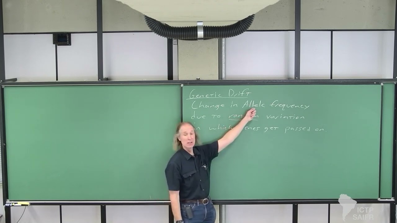
Genetic drift is the stochastic change in allele frequencies caused by finite population size, modeled using the binomial distribution and the Wright-Fisher model; it leads to random fixation or loss of alleles over time, with the probability of fixation equal to the initial frequency (for neutral alleles, this is 1/(2N) for new mutations), and the average time to fixation being approximately 4N generations, while heterozygosity decreases over time as genetic diversity is reduced through this random sampling process.
Genetic Drift in Evolution: Causes and Mathematical Modeling
Added:Fundamental genetics concepts, including alleles, genotypes, and the calculation of allele frequencies in a gene pool.
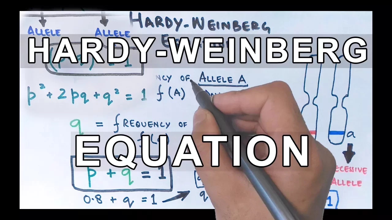
The Hardy-Weinberg Principle, specifically how it serves as a null model of evolutionary change assuming an infinite population size.
Basic probability theory, including random sampling, independent events, and the binomial distribution.
The concept of Effective Population Size (Ne) and how ecological factors like population bottlenecks and founder effects reduce genetic variation.
The Neutral Theory of Molecular Evolution, which posits that most evolutionary changes at the molecular level are caused by genetic drift rather than natural selection.
Coalescent Theory, a mathematical framework that traces the genealogical pathways of gene copies back to a single common ancestor.
The interplay between genetic drift and natural selection, understanding how population size influences which force dominates evolutionary dynamics.
1.8K views91likes1:05:36Original Release: 2023-11-16
[Music] [Applause] [Music] [Applause] [Music] [Applause] [Music] [Applause] [Music] [Applause] hello everyone welcome back to the channel if you're new here I'm Zach Hancock I'm an evolutionary biologist who specializes in population genetic gencs phenetics and genome Evolution and this is the fifth episode of the causes of evolution series my ongoing Series where we look at the quantitative aspects of evolutionary theory and we really try to derive all of the mechanisms all the evolutionary forces from sort of first principles in mathematics um for regular viewers um you'll know that it's been a little over a month since I last published a video which is a little bit of a long lull for my part I've been really really busy in the lab lately we've got two papers we just submitted um on top of me going through a lot of the genome sequences that we finally got back um for those of you that might be familiar with my amphipod sequencing project that I've been sort of documenting on this channel a little bit um we finally got the genome sequences back for that and I've been kind of combing through them and doing some quality control stuff like that so I've been just really really busy in real life um so but I'm you know I'm really exced exced to be back talking about this topic genetic drift is one of my favorite mechanisms of evolution and it's also one of the most misunderstood mechanisms of evolution so really excited to kind of get into the nuts and bolts of how it works um and we we always start these this uh these episodes off in this way talking about the assumptions of Hardy Weinberg you've seen this many times if you've watched the previous episodes um again we we bring this up because all of the mechanisms of evolution are derived from violations of these assumptions so the previous one are the gametes are paired at random we know when they're not paired at random we call this non-random mating this is a pretty weak evolutionary Force if you recall it doesn't generally lead to sustained change on its own but it can change a little frequencies uh and it can change genotype frequencies as well so um it is an important force of evolution but it's a pretty weak force on its own um the second is that gametes aren't preferentially chosen from the gene pole and when they are preferentially chosen that's natural selection right it's selection is peeking into the bean bag and picking the best ones um we went through and derived all the mathematics behind at least one Locus models for natural selection um we then discarded the third one a little frequencies are equal between the Sexes violations of this is actually not a mechanism of evolution because a single generation of random mating actually puts you back into Hardy Weinberg um the most recent one that we did was looking at alals um the violation of the assumption that alals don't change from the individual to the gene pole that's mutation right that there's not some new variant that emerges um and is introduced into the gene pole um we talked a lot about um sort of like the the biochemistry behind mutations the mechanisms behind mutations um and then a little bit of sort of the pop gen Theory there today we are looking at the fifth violation um and that is that gametes are drawn infinitely and with replacement and when they are not drawn infinitely and with replacement that means we're actually looking at a finite sampling scheme and that is what we call genetic drift so let's start off pretty simply and let's just like take a broad view on what the effects of finite sampling are now I'm going to talk about this in terms of like populations and alal and stuff but really this applies to any kind of statistical sampling in which you have a finite number of possible samples to take right where you don't have an infinite sample Choice um so this is so this is true in many many systems not merely in population genetics so let's start off with um a population of size 10 right so there's 10 balls here five are blue and five are red now let's imagine that each one of these individuals produces an some number of gametes and we take those gametes and we put them into a bag right um and all of the the distribution of gametes within the bag should reflect the number the proportion of Reds and blues that we had in the preceding generation right so there's 50% of all the you know beans in the bag balls in the bag are blue 50% are red I'm referring to beans in the bag here and I've included the little halane uh Cartoon um to kind of draw an illusion to uh a paper that he wrote in ' 64 called uh defense of bean bag genetics if you if you've never read it I highly recommend you go check it out um it's a it's a satirical and really funny paper um that sort of uh fighting back against some other biologists namely erns Mayer Who were critiquing population genetics by calling it bean bag genetics um and so check it out it's a really funny paper but this is sort of a simplistic way to to think about this process is that each one of the par parents give some number of gametes into the bag and the proportion of gametes in that bag reflects the preceding um the distribution of the preceding generation okay so now what we want to do is we're going to pick 10 gametes out of that bag and the 10 that we pick are going to populate the Next Generation okay and we're going to pick them at random and since we only pick 10 right and we're not drawing infinitely from that bag that means that by chance alone what we pick might deviate from the proportion in the preceding generation so to make sure that I did this like as randomly as possible I created an object in the programming language r that I just called X and I set that equal to um uh C just means include everything within this so this is five zeros you can think of these as blue and then five on which are red and then we use the function sample we sampled the object 10 times with replacement this is really important so what replacement here means it's a statistical term saying that let's say we drew a blue right by drawing that blue we could technically have changed the distribution now of Blues in the bag right so if we just take that blue out set it aside now we've changed that distribution but sampling with replacement means that we take the blue we mark down we got a blue and then we put it back right so we're keeping the distribution in the bag exactly the same what that means in a biological sense like what that assumption would mean is that each one of the parents can produce effectively infinite gametes right that if we choose one of the gamet that they produced that doesn't dramatically change the distribution of gametes right so we still have the same number of Blues still have the same number of Reds in the bag um because they produce so many gametes this is generally a fine assumption because organisms do produce lots of gametes right so that's why early population geneticists were perfectly fine with that assumption because organisms do produce lots of gametes um where that starts to become problematic is if you have things like gtic selection right you have some other sorts of biases that are impacting how many gametes an individual might produce but in this case this assumption works perfectly fine so that's that's why we're talking about sampling with replacement it's important to sort of bear that in mind um okay so we're we draw them from the bag and what I ended up getting is in the Next Generation we have 40% blue and 60% red just just by chance we have now changed the distribution of blue and red by 10% and then we do it again so now all I've done is I've taken the new distribution of Reds and blues the 40 and 60% and then I make I remake the X object as four blues and six Reds and then I sample from that bag right when I do that now suddenly in the Next Generation we have 30 30 % blues and 70% Reds right so again that just by chance just by chance sampling we are changing the distribution of how many gametes are going to be given into that bag so this is again a very simplistic way of thinking about the effects of finite sampling now one of the useful ways of thinking about genetic drift is and replicates so if we had if we did this exact same thing many many times for a bunch of replicate population so in this case we've got five different bags so five different populations where we're starting off with 50% blue and 50% red and then we're walking every single generation and seeing okay how does it change so what I've done here is I basically did that same process I just walked you through but I did it five times in replicate and I did it until either blue or red are the last things left in the population right so starting here after one generation of sampling we go from Blue to 40% red to 60% do it again red is 70% blue is 30 the next generation it stays exactly the same the I drew the same distribution and then after one two after four generations red is now fixed in this population okay so for this replicate red becomes the only Al left and this one you can see it took a lot more generation so there's a lot more fluctuation but eventually blue fixed in this one red in this one red in this one and then this one had the most number of samples that I had to walk through before eventually blue became the one that was fixed so in our five replicates we see three out of the five times red fixed two out of the five times blue fixed um that's as close to half and half as you can get in this in this uh setup right um so again that's just a random fixation of which ones are going to end up being the last Al in the population and that's just a very simplistic way of thinking about the effects of finite sampling um this is a plot of 10 different replicates all starting off with a Leal frequencies of 50% um going out to 50 Generations after which you can see all of them have been fixed and you can see it's super noisy right so they're just these Al are just bouncing around some of them fix really rapidly some of them are lost really rapidly some of them bounce around for a long time before they go to fixation or law so this is the same thing that I was showing you previously but just showing it for lots of replicates across you know up to 50 Generations right okay so the stochastic change in a little frequency every single generation is genetic drift that's what we mean by genetic drift and we've we've now kind of looked at it very simplistically just sort of like you know we're just drawing beans from a bag but we can actually evaluate this probabilistically and and that's generally the way in which we approach genetic drift is because since we it's not deterministic like mutation or selection we have to kind of approach this in a probabilistic manner and since the way that we've been approaching it is as in a bolic state so we've got Reds and blues for example um you can also think p and Q right as the frequencies of red and blue um since there's only two choices we can actually model this using the binomial distribution the binomial being two right um this is the same sort of distribution you would use to model a coin toss right because you can get heads or tails uh it's binary zeros and ones right that's the binomial distribution and this is the way it's set up so we say the probability of having I number of Al of B uh is equal to 2 N choose I that's the way to read that um where 2 N is the total population size and then I is again just the number of bels that you're asking what the probability of it will be um multiplied by P which is the frequency of the blue alals in the preceding generation raised to the number that you expect to choose multiplied by Q which is the frequency of the red in the preceding generation raised to 2N minus I so since there's since it's by alic if you chose I number of blue alals then you must have chosen 2 in minus I red alals let's put some numbers into this just to kind of make it a little bit clearer so let's say we wanted to know what's the probability that I had five Al of B in the Next Generation now remember we started off with five and five so that's basically asking what's the probability I stayed exactly the same um so that is equal to 10 factorial because the population size is 10 divided by 5 factorial * 5 factorial it's five and five because again we're asking what's the probability of getting five so that's the I here and since we're getting five of the B and the population size is 10 then we must have also chosen five of the red right and what these factorials indicate is to perform the following operation so for like five factorial is equal to 1 * 2 * 3 * 4 * 5 um and what this represents is how many distinct possible States could we have chosen so we're assuming that if we chose five that's an independent event of whether or not we could have chosen one or we could have chosen two or three or four right so we need to we need to multiply all of those possible choices together to be able to get the probability that we chose exactly five instead of any other number up to five so that's what this first part represents and then the P's and the q's here are 0. five because that's the starting and then raised to the number of choices right um and then plugging in our numbers we get the probability of choosing five Al of B is equal to 0.246 roughly 25% so uh to sum up that basically Bally means that we have if we you know start off with five Al of B what's the probability we have five in the Next Generation it's 25% and we can do this for any number of alals going from loss all the way to fixation so we could ask what's the probability that I have 10 alal of B right that is to say that b goes from five to 10 in the Next Generation so from 50% to fixed that's that we just plug in those numbers here and we see it's a very low probability that you started with five and then jumped all the way to 10 same thing for if you have you know only two Al of B right we can plug in any number from 0 to 2 N and ask what that probability is um and then we can plot that probability distribution like so so on the x- axis here is the number of beils that we're going to choose in the Next Generation again it's conditional on how many we started with is is how this probability is calculated but on the y- axis is then that probability right so you can see though with the highest probability we stay at exactly five we stay at what we started with um and then that that distribution start to fall off as we get closer and closer to either loss or fixation it's actually symmetrical it's the same probability in either direction right um so highest probability we stay exactly the same but it's only 25% right so there's still a very good chance and and you know 75% chance that you're going to change in a frequency right despite the fact that staying the same itself has the highest there is a greater distribution outside of that and so more than likely you're going to to change in a little frequency by chance alone um another thing that's important here is how tight this distribution is is completely dictated by the size of the population right so how big this 2N is is going to dictate how broad this distribution is so if you make 2N really really large this distribution gets really really narrow right so and in fact if two in goes to Infinity then the distribution is exactly centered on five and it will never change and you would be in Hardy Wineberg right um and so like the the further and further you get from Infinity the broader that distribution is going to become right so just bear that in mind as you're thinking about genetic drift and um the probability of changing that that alal is a function of how many samples you're taking every generation okay so now we've talked about the very simple what are the effects of finite sampling in a sort of bean bag way and we've introduced the binomial distribution now we're ready to talk about the very first model in population genetics for looking at finite sampling and that is is looking at genetic drift and modeling it in a population genetic framework and that's the right Fisher model um so the bearded man here is RA fer and then the man next to him is Su Wright and the two of them together um were the first to use this sort of binomial distribution in a matrix algebra approach which we'll talk about in a second to actually model how Gene frequency should change through time using just from just finite sampling or just genetic drift um it's the simplest model of genetic drift it basically has all of the assumptions of Hardy Weinberg except for the finite sampling part uh and we'll make That explicit so you can imagine um in diploid parents that produce an infinite number of gametes right so there's we're sampling with replacement um and then they pair at random right so we have completely random mating um individuals are assumed to be hermaphroditic and what this means is that they actually have a probability that they can self right and that probability is equal to to one on N right and so you can think about it as if they're mating at random then they're just picking some individual in the population at random to mate with and by chance a one on in they could pick themselves right so that's sort of implicit within the model here um you should recognize this expression as just the binomial distribution right this that's all that this is um and this x sub i j represents a transition Matrix between states J and I right um and so the XI J is the probability of being in state I at time t + 1 given that you were in state J at time T I know that that that's maybe some difficult jargon but I'll explain exactly what that means in just a moment um but this very simple expression which is effectively just the binomial distribution viewed through a transition Matrix um is the right Fisher model right and let's walk through how exactly it works so let's start off uh by calculating the probability Matrix itself so up here at the top is the number of alals of B we'll say we'll stick with the blue alals um which will be equal to J so that's the J and our transition Matrix so you can either have zero where there's no alals um or you can have four where it's fixed and we're setting two in equal to four here just to make it simple because as you get to bigger and bigger and bigger population sizes this transition Matrix gets enormous right and so I'm justy to limit it such that it can fit on a slide and we can do them we can completely do the math um in in a much easier way so 2 N is equal to four uh instead of 10 we're 10 my gosh it would take us forever to do 10 so 2 N is equal to four and at generation T so the present generation how many of the be do you have and that's equal to J okay so that's on the rows and then the column here is at generation t+ one so in the Next Generation the number of Beals you have is equal to I okay okay so let's see how you would read this so let's say we started at generation t with zero alals of B and the Next Generation what's the probability we have zero alals of B right and so if we started with zero what's the probability of one 2 3 four and then if we started with one what's the probability we have 0 1 2 3 4 right so that's the way you kind of read this Matrix um importantly if we start with zero alals right and there's no mutation like right there's no other processes happen if we start with zero alals and the probability in the Next Generation we have zero alals is exactly equal to one right because there's no mutations bringing that alil back and so if it has been lost then with probability one it will stay lost um alternatively if it has been fixed where everybody has it over here at four then the probability is one that in the Next Generation everyone will still have it and we call these two states in the transition Matrix absorbing States because effectively everything between there is some number less than one because that Al is just you know going to be fluctuating around but then once it falls into one of these absorbing States either fixed or lost then the system basically ceases right you you are now fixed or You've Lost That Al and you're finished iterating at that point so that we call these the absorbing States everything else in between we fill in with the probability so let's say we started off with one Al and we want to know what's the probability in the Next Generation that we have none to say that's effectively that that little little has been lost well that's a 30% chance all that we've done here is we've just plugging in these numbers into this expression right that's where all of these numbers are coming from they're coming just straight from this expression here where again 2N is equal to 4 the I is equal to how many we're going to have here and then the J is equal to how many we started from up here right very simple we're just plugging in the numbers so we can fill in the rest of this Matrix with um with depending on what we started with in J and what we're going to end up with an i okay so that's our probability Matrix you know real simple we can get that those calculations um but that doesn't really tell us how we could iterate in like a population model right so like what the right Fisher model really wants to do is iterate over many generations how do we expect a frequencies to shift we want to be able to predict that right so that's and Akin to asking what's the probability of having exactly ials of B after T Generations right so let's start off by assuming we begin with two be where 2 N is equal to four so so the Bel starting off are at 50% frequency this is the new Matrix that we basically are going to want to build here the columns are going to be generations and then the rows are going to be the number of Beil so starting at generation zero we have exactly two Al right um so generation zero with exactly one probability because that's what we we're starting with we know what that is and so with zero probability we have any other number because again we're we're stating we're starting with two um and so what we want to know is okay in the next generation at time one how many alals do we expect to have um one of the things that this Matrix is going to have to follow um just to to kind of make this explicit is that for every single one of these columns um the sum of those columns must be equal to one because it is a probability um and so we basically just write that like so so from J equals zero where there you know it's lost up here to 2N which is four down here um we sum across Y and we're calling this new Matrix we're creating we're going to call it y we sum across the Matrix y subj of T um for every value in the column uh the summation of which must be equal to one so at zero we know obviously it's going to be equal to one but at every single one of these changes it's always going to end up being equal to one um okay so how we how are we going to calculate this what do we need to do well we need to bring back our our other Matrix right um and then we're going to do a little bit of Matrix algebra here to enable us to be able to calculate every single one of these Generations across effectively an infinite number of generations right so I put the little equation up here this is y1 where this is the column uh for y1 is equal to X where X is this Matrix multiplied by y not where that where y not is this column okay um and we're going to do a little bit of Matrix algebra to be able to calculate the change in the frequency every generation okay so I've color coded these to kind of help us keep up with things so the blue is always going to be what we're multiplying from the Y Matrix the red is going to be what we're multiplying from the X Matrix and effectively again the the product of these two is what's going to be the entries in each of the new columns that we're yeah in each of the new column that we're filling out for the uh the Y Matrix okay so this is how we do it we want to fill out that very first entry and so what this first entry represents is the probability that we have no more of the blue Al okay so we need to then multiply all the possible ways that we could end up with no blue alals well we could end up with no blue alals because we started with no blue alals up here so that would be one multiplied by zero because we know we didn't start with no blue alals but just just to keep up with everything so that's written down here so 1 multip 0 is the probability we started with none and then we have none in the Next Generation plus the probability that we started with one and then have none in the Next Generation again that's 316 that we started with one and have none in the Next Generation since we know we had two and not one that's also multiplied by zero right then we have the probability that we started with two and went to 0 which is 063 so that's the probability we started with two went to zero multiply by how many we started with right well in this case we did start with that many and so then we have 063 multipli by 1 right and you can see the rest of the entries are also zero because the rest of these entries are zero and so the probability that we started with two and went to zero right is 063 and then we basically just do the same thing for each and every entry so for this one here this is again the probability we started with zero and then went to one is zero right and the same thing is here so that's just 0 * 0 um plus the probability we started with one and went to one or stayed at one again is going to be multiplied by zero because we didn't start with one right so this First Column is really easy to fill out because we know we started with two and not these other ones okay so let's just go ahead fill that one out that one's really simple to calculate because again we already knew what the preceding values were and so most of the multiplication was just zero now that we've gotten that generation in though the next gener Generations calculations are a little bit more complicated cuz now notice we are no longer looking at this column to calculate for Generation two we are actually now going to use this column okay so for to calculate Y 2 so this is this column is equal to once again X multiplied by the column y1 which is what we just calculated so now what's the probability that we have zero alals well that depends on how many we started with if we started with zero what's the probability we have zero well that's equal to one so we multiply 1 times the probability we started with zero which is this value here plus the probability we started with one and went to zero which is this multiply by this which the probability we started with one right and we do that all the way across for each one of these values and we end up with the probability of having zero alals in generation 2 as. 166 okay then we do this same thing with the probability of having one Al right and we just follow it through once again right and then we do that all the way through the rest of the Matrix we can fill that Matrix out to Infinity right um there's a couple of interesting things uh should emerge from this pattern so notice first that we started off with two right so that probability is obviously one and the first generation that probability stays high at 375 and where the other probabilties around it are lower so you can remember that sort of bell curve where you had highest that you stayed the same and then it begins to fall off but then watch what happens as we iterate through more and more and more Generations that probability starts to flatten right so it goes from 375 to0 246 to 181 to.
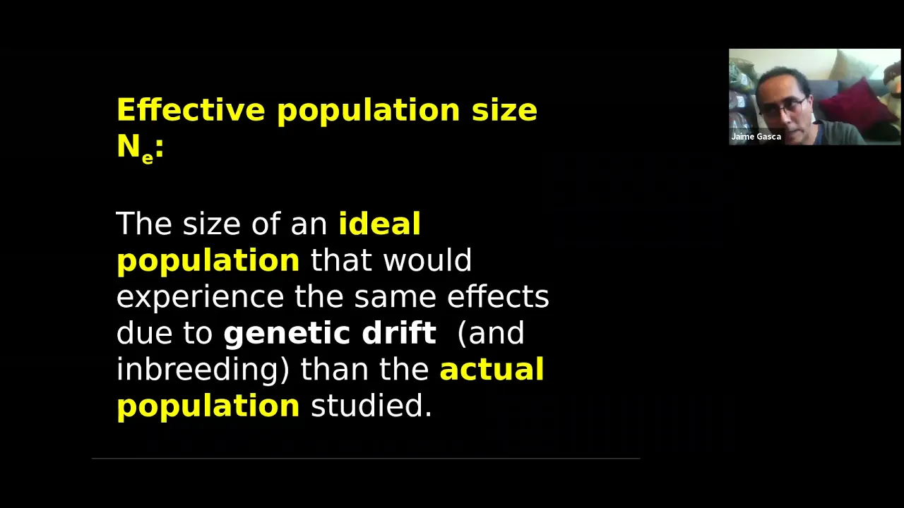
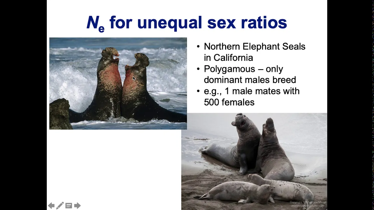
136 right so it's getting so the middle part is getting lower and lower and lower and then watch where that rest of that probability is being added to it's being added to the extreme values right so they're starting at the lowest but then by the time we're only four generations in they are now the higher probabilities right so you have a higher probability by Generation 4 that you have either lost or fixed that Al so what that distribution is looking like is it starts off like this and then it flattens and then the ends start to rise right um and then if you go all the way out to Infinity what you will find is that with a 50% probability you have lost 50% probability you have fixed it and all the other ones in between are basically zero that is that that it is still polymorphic is effectively zero so this really drives home the central point of genetic drift the genetic drift leads to the loss or fixation of an Al and that the probability of fixation is equal to its initial frequency in the population so notice this we started off with two right and since the population size is is four that's a 50% frequency and so the probability notice that it goes to fixation is exactly 50% that also means that the probability of loss is one minus the starting frequency now since we started with 50% the probability of loss is exactly equal to the probability of fixation but if we were looking at say a brand new mutation in the population right brand new mutation start out at frequency one on 2 N because there's only one of them out of all possible individuals so the probability of fix of a brand new mutation then under just genetic drift alone is one on two in right and that's what we've shown here using the sort of Matrix algebra approach you've probably heard this many times that the probability of fixation is one on two N I know I've said it on this channel a bunch of times um but this is where that math actually comes from um furthermore that tells us that the probability of loss of a brand new mutation is one minus one on 2m um hence most of the time brand new mutations are lost lost a chance and the probability that they are lost a chance obviously increases as the size of the population increases um and the and the probability that a mutation goes to fixation by chance increases as the size of the population decreases right so that kind of tells us something about why population size is such an important feature of genetic drift is why it's dictating the rates at which alals can rise and fall in free frequency just due to chance alone because this chance alone is a stochastic sampling effect okay so let's add another column here this is something else that's really interesting and worth digging into is that the average frequency of an Al is expected to stay exactly the same across Generations this might seem counterintuitive but if you can imagine this as again as a replicate population so a bunch of bags instead of just a single population and we consider each one of these columns again as the probabilities which would be shared across multiple populations then uh P bar so the average frequency at time T is equal to the initial frequency that we started iterating across every possible generation right so to so for example let's say we wanted to know what the average frequency should be at generation one right so we would get that by saying okay the probability we have zero alals multiplied by the number of alals we have then the probability we have you know one Al multiplied by how many we have and we just do that across the whole column that's the summation across the whole column and then we divide that by the number of possible alals 2 N and in this case four we can see that that's equal to 2 over 4 which is equal to 50% okay we could do that for every single column all the way to infinity and what we would find is that the average frequency in each one of these iterations is exactly 50% it doesn't it doesn't change across Generations um and this is true irrespective of when they start going to fixation so let's say you have 100 populations right half of them are going to fix the alil by Chance the other half are going to lose the alil by chance so the average of those two is still 50% since 50 fixed it and 50 lost it right um so that's another kind of interesting feature of genetic drift um furthermore the variance in this uh average is based on the binomial distribution variance um so the variance in the change in P across Generations is equal to P 1 minus P divided by 2N what 2N is the the total sample size um this is a really important equation uh when it comes to like calculating the effective population size which we'll touch on a little bit uh towards the end of this um the next column I want to add is heterozygosity um and this is a really really important feature of genetic drift as well that since genetic drift always leads to fixation or loss that means that every single generation what genetic drift is doing is it's reducing diversity right it's it's removing variation from the population um and the rate at which it does this is a function of the population size so if we're calculating hetro zygosity here um you should actually kind of recognize this form if you think back to Hardy Weinberg um this is just 2 * P * Q that's what these two terms are it's it's it's 2 PQ where we're just summing over all the possible ones from loss to fixation and then across each column when you plug in the numbers here you can see we start off um at generation zero at heterozygosity 50% it's just equal to the that initial frequency and then as we walk Generation by generation you can see the heterozygosity goes from 0.5 375 281 all the way and then by the time you get to the infinite time point heterozygosity zero because you've either lost or you fixed that AAL there's no more more diversity in the population so genetic drift always reduces heterozygosity um another thing that we can ask is how long uh should we expect to wait until an alil becomes fixed in a population there's two different approaches to this problem one is very um cumbersome and people don't generally do this but it it is an exact measure so you could do it this way and it's again using this sort of Matrix algebra approach if we ask okay so this is the time to fixation of p is equal to 1 over P the summation from or multiplied to the summation of t equal 1 so starting off at time point1 all the way to Infinity um and then T multiplied by what is the present column summation uh this is y sub 2 N T minus the previous generations one so you can see it's kind of an iterative uh it's it's an iterative formula starting at time point1 going all the way to Infinity um that's obviously a very cumbersome way to calculate this because that just basically means you have to calculate the entire Matrix right um people don't generally want to do that uh and so what we actually use whenever we're doing this calculation um is we often rely on What's called the diffusion approximation the diffusion approximation which I haven't talked about in this series yet but we will once we start kind of putting together a couple of processes um is actually borrowed from physics um so it's a it's actually about gas molecules diffusing in a vacuum and so you can actually apply this to population genetics uh Cura was one of the first to do this actually um and the way you can do it is you imagine like you've got gas particles moving around in a vacuum and their their movements are random right which can kind of mimic genetic drift so imagine if you just flattened that plane you started all the particles at at one side and that's you know the initial frequency starting them at one side and then you let them walk across that plane until they get to the end where the end is fixation so their movements are random and they just kind of bounce around right just like a particle would diffus through a vacuum right and we're just conditioning on that diffusion being one directional so with those kind of modifications to the diffusion approximation we can actually use it to calculate lots of interesting things about you know stochastic processes and population genetics um and this is one of those interesting findings so we can see that the the the time to fixation of p is actually equal to this little expression here and what's really cool about this is that when p is very small such as like when it's a brand new mutation in a population um then this actually simplifies to approximately 4N right so this is another thing you've probably seen many times both myself and others have have said that the average time to fixation is 4 in Generations this is where that comes from it comes from the diffusion approximation and assuming that the starting frequency of p is very small such as in the case when it's a brand new mutation um so we can actually plot this shown here um this is again just keep keeping the formula here so this is the average time to fixation um and down here is the frequency of p and then on the Y AIS is the age of the AL right so how long how long has that alil been segregating in the population before it goes to fixation and you can see for a population of size 1,000 um that the average time to fixation is 4N Generations I've just marked that here by this dashed line um because of this this allows us to actually calculate the age of any natural Al that are segregating in a population um because it has this sort of expected um rate of increase in frequency we can we can get a pretty good estimate of how long it's been segregating based on what its frequency is in the population and again assuming that it's that it's a neutral mutation one of the things that's really cool about this is that if you look at the change in the frequency across Generations it's nonlinear right so it's not like it's a linear increase it's actually most of the change in the frequency or most of the time to fixation are actually uh concentrated when that Al is at low frequency so over here you can see that you know halfway to fix or halfway of the time to fixation would be 2,000 generations and you can see that that is only maybe 25 30% frequency so half of the time of that Al's life is spent at low frequency it takes a really long time for it to start in increasing in frequency but then once it starts you can get an almost linear fit by the time you're at about 50% frequency right um so again because of this we can calculate how long that alil has been around based on its frequency so for example let's say um let's use a human population as an example and let's say there's some alal that's at 80% frequency right so it's really really high frequency if the population size is 10,000 uh using this expression then that Al first emerged 35,000 th Generations ago um for a human generation time that's approximately 892,00 years um so for any Al that are at really really high frequency in the human population they are probably very old now they're very old specifically if they're neutral right if they if they're if they've risen to that high frequency completely by chance alone then we know that they're very old right so we do have to distinguish between alls that are at high frequency because selection is driving them versus alals that are at high frequency because drift is driving them and there are really cool ways we can tell the difference between those two things which we'll get into in future videos um I also just wanted to juxtapose uh this with what is called the site frequency spectrum so over here on the right um the x axis is the alal frequency starting at you know basically one which is you know only one individual and the population has it all the way to 50% um this is what's called the folded site frequency Spectrum so we're not showing you know all the way to fixation we generally uh truncate this distribution at 50% because it's very hard to distinguish uh whether it's ancestral or a derived AAL so we usually just break it into 50% and this sort of distribution to me really helps demonstrate the process of genetic drift right that most alals in populations that are brand new are at you know very very low frequency and most of the time they never increase in frequency right so you can see most alal that you would find segregating in the population are down here at very low frequencies and then as you get to higher and higher and higher frequencies that number just exponentially falls off to where most alals have already been lost right so very very few mutations that ever emerge in a population will ever reach high frequency um so I just wanted to kind of show that this is like a the neutral expectation of the AL frequency spectrum is is this shape where most Al emerge and are lost by chance okay so all of this is maybe seems very abstract there's lots of model assumptions um you might be thinking how often can any of this actually be used to model real populations right like like this is a very seems very abstract and mathematical um but it turns out it actually works incredibly well on real populations and this is a famous study from Buy in 1956 it is a laboratory population but the fits um to this binomial distribution are incredibly well um so what buy did is he examined genetic drift and laboratory populations of dropil melanogaster which is a the you know fruit fly and he was looking at populations that were heterozygous for the BW Alo so starting over here this is the gene frequency distributions um at generation one for all of his replicate population so it had a bunch of different populations and this is the distribution of that frequency um at the beginning of the experiment and then what he did he just kept the population sizes you know roughly the same and then across subsequent Generations he just measured okay how many what's the Le frequency in the Next Generation and then he just plotted that all the way to generation 19 notice what's happening so he starts off with this sort of binomial distribution this very like you know bell curve distribution and then at each subsequent generation it starts to flatten right you can see as he's walking through all of these Generations it flattens and then it starts to spread towards the edges so by the time you get generation 19 you have lots of populations that are you know fixed now for these for these alals um which is exactly what we predicted using just the simple right Fisher population model that is just based on the binomial distribution right so this is pretty incredible that you will that you see the exact shape that we expected to see furthermore he estimated heterozygosity as it changed through subsequent Generations in the experiment um the little dots here are the measured what he actually empirically measured in terms of heterozygosity and then the dark line is the fit from the formula that I showed you previously for calculating heterozygosity look at how remarkable that fit is right and again that formula for calculating heterozygosity is assuming this binomial distribution it's assuming all of the all of the assumptions that we made previously and despite that the fit is very very good um one of this is one of the key reasons that I like to always try to bring back this empirical application is that people often like to say well it's you know this is bean bag genetics right like there's there's so many assumptions this can't possibly reflect anything in reality but all of these models are actually exceptionally robust to these assumptions um and it's very important that we understand that uh and so that's why I wanted to show you this this you know sort of classic genetic drift experiment that actually almost exactly replicates sort of what we were looking at um in in the you know simple math leading up to this point okay so the next really important thing to understand is the relationship between the concepts of genetic drift and inbreeding um inbreeding in this context um simply means that individuals are identical by descent okay that they that they share a common ancestor um this is not IM breeding in the sense that relatives are choosing to mate with each other it just simply means that you are identical by descent so if I have a certain Al and you have that exact same Al and that's because we share an ancestor that had that Al at some point in the some point in the past then we are inbred with respect to that alal okay that's that's what inbreeding means in a population genetic framework and we can measure this using fstatistics so I introduced the F statistics in The non-random Mating uh video previously um and it's basically just a measure of the probability that any two individuals are identical by descent and to to kind of make this clear so imagine the simple population where again you have red and blue alal um and let's assume that if you are blue then you are identical by descent at some point in the past and if you are red then you are not okay so for these two individuals since they have this common ancestor they are identical by descent right they come from this single ancestor in the preceding gener generation the probability of that is one on to M right that's the probability that each of these chose this ancestor out of the two n possible ancestors they could have chosen right so that's the probability that they are IBD um again this tells us something really important and that is that the probability of being identical by descent scales with the size of the population smaller populations are more inbred this is this is what we mean when we talk about inbred populations that the smaller and smaller they are the more likely that they are composed of close relatives right and close by close we mean how many generations back that you share an ancestor with some individual right so these individuals are identical by descent now notice these two individuals right they are both blue so they are identical by descent but not in the preceding generation so we call this identical by state right and so if you're identical by state we're assuming that you were identical by descent in some preceding generation so we have to go back a little bit further before the two of you have a common ancestor okay um or you can be not identical by descent so if you are like the red and the blue here then you are not identical by descent and that occurs with a probability of one minus one on 2m so in the preceding generation you didn't choose an ancestor and then in no other preceding generation are you related right um so given that these are the different ways that you can be identical by descent or not we can then measure that probability that you are IBD and that is effectively what the f statistics do so we can Define that at F subt that is what's the probability you're identical by descent in the present generation that's equal to one on two in that's this part here plus the probability you are not identical by descent one minus one on two in multiplied by the probability you were identical by descent in a preceding generation which is this component here right now what we can then do is a little bit of algebraic magic um and we can actually simplify this down into a very simple recursion equation that will permit us to predict across many generations so we do this by first um multiplying each side by negative 1 that's permits us to do a little bit of rearranging and then we add back in plus one um and this gives us this expression here where 1 - F subt is equal to 1 - F subt minus 1 so that's the preceding generation component multip IED by 1 - 1 2N what we can now do is proceed starting at tal 0 and then go to T so go to whatever generation into the future we want to go to and all we need to do to be able to calculate that F value uh that probability of being identical by descent is just raise the second term to T right so how many generations do we want to iterate from when we started to when we ended and what's really important about this is that as T gets lower large so the longer the more Generations you iterate over that F subt goes to one okay so that the probability that you are identical by descent as T gets large goes to one what that means is that everyone in the population is IBD they're identical by descent the longer the more Generations you iterate over that probability becomes one guaranteeing everyone will eventually be related to each other other and this occurs at a rate that is the reciprocal of the population size one on two n so again the smaller the population the faster it is that everybody shares a recent common ancestor big populations it takes longer for everyone to share a a single common ancestor right so that's that's what genetic drift and and using the sort of idea of inbreeding statistics for the like the F statistics tells us is that eventually everyone will be identical by descent um and this leads us uh very nicely into the next Concept in genetic drift and that is coalescence so this idea about being identical by descend we're kind of iterating forward in time right we're thinking about we're walking forward in time at what point is everyone related coalescence looks at it the reverse way so starting at the present day and then walk looking backwards how far do we have to go until everyone is related so since we know the forward in time guarantees relationships the backward in time does exactly the same so let's see if we can link these two ideas together so let's start off at generation zero um and say there are 10 lineages um and each lineage is just represented by colors okay um and then notice that by T equals 15 so going down this direction there is only one lineage left and it is orange okay so walking in that direction what we would say is that forward in time the orange lineage has been fixed everyone in the population is now identical by descent all right backward in time if we start off at the orange down here and then we say okay at what point does everyone in the population have one and only one ancestor um we can see that these lineages eventually coales in into this one starred individual at time point two now this tells us a couple of really interesting things first is that forward and time uh models keep account of all lineages right every single lineage they keep account of from every single generation despite the fact that the majority of all of those lineages will not contribute any genetic material to the modern day right so here we had a bunch of lineages right but only the orange one ends up being the ancestor of everyone alive if you were looking forward in time you're keeping up with all of them right but if you are going backwards in time in the coalescent approach you're only keeping up with lineages that actually contribute to the modern day this makes a lot of the coalescent models a lot simpler and a lot more tractable than the forward in time models where you're having to keep up with individuals that are never actually going to leave Offspring to the present day it also shows us something else is that in a coal framework right the last common ancestor of the population is just one individual that existed in a population right so though we know that we started iterating at time point zero you know back here this is actually the most recent common ancestor of the current population this individual had an ancestor like this is their ancestor and we also know that this is that this generation is not when this population emerged so this tells us a couple of important points um that we should always bear in mind is that coalesence is not origin of the population so just because we say you know the coalescent ancestor the most recent common ancestor lived at this point in time that says exactly nothing about when the species emerged or when the population emerged it only tells us when at what point into the past is everyone identical by descent right right that's it that's all that it can possibly tell us to get the origin of the population the origin of the species we have to compare to some other sister taxa right that will allow us to get you know closer to that answer but just a coalescent analysis in a single population will not get us that answer okay um and again this the starred individual is not the only individual alive there are many other individuals alive the population size has not changed right it's exactly the same population size Through Time but as we've shown previously the the way genetic drift works is that it guarantees loss or fixation so there will always be either the lineage will be lost or it will be the only lineage around that's what genetic drift absolutely guarantees us okay so another thing to bear in mind is that for each generation the probability of coalescence is one on 2 N because remember this is just genetic drift right so going backwards in time we're saying what's the probability that you came came from exactly the same ancestor well that means that you picked one out of two impossible ancestors so that's the rate of coalesence backwards in time um the average time that we should have to wait for two lineages to coales is then um T Lambda is equal to 4 n / I IUS one where I is the number of lineages that we're asking are going to coales if there's only two lineages right that we're looking at then the average time to coalescence with two lineages is two in Generations as we add any number of lineages right as the number of lineages gets large um then the average time to fixation of all of those lineages approaches for in which again brings us back to the previous slides where we were talking about the average time to fixation being 4 in Generations um this also tells us something really important about the shape of coalescent trees right um and so what it shows us is that as we sample more and more individuals in the population that is say as I which is the number of lineages we're sampling gets really large most coalescence is going to happen rapidly it's going to happen rapidly and really early on um and that's what's being shown here in this tree so we start off with six lineages and then by time uh T of two up here we only have two left right and most of it most of the lineages have been lost by by this line so there most of them are are truncated really early on and then you get long lineages backwards in time so on average half of the waiting time for coalescence is in the last two lineages right so remember 2N is the average time for two lineages to coales and so for any number of lineages most of the time that you're waiting for the last coalescent event is in the last two lineages um and again just to really drive this point home drift ures population-wide IBD will be reached there will always be one ancestor to any population um that is what genetic drift ensures okay so sort of the last concept I want to touch on is the effective population size this is a concept that is um deeply misunderstood not just in the general public um who maybe don't even consider this idea but it's it's misunderstood among a lot of biologists like if if like non-population geneticists people that don't work with this idea a lot um really struggle to understand what it means and what it's actually measuring um but it's a super important variable because just like with mutation we had mu mu was our value for selection we had s right so for drift our our sort of measure that's important is population size right um but some interesting things can happen in the Dynamics of empirical systems that make the um population size not a good reflection of the variance in alal frequencies so let me let me give sort of ort of a a mock hypothetical empirical example okay so imagine you were working on gorillas you're working on a population of gorillas and you know because you've you know been studying them for many generations and you've counted up how many individuals there are you know that the census population size of this population of gorillas is a thousand okay and then you go out and you measure the frequency of some Al right that you think is neutral you think it's just you know neutrally changing in the population and you measure the frequency of that Al as 6 okay um starting off and then you measure it again over subsequent Generations right so you you measure it once and then every single generation you measure it and what you find is that the variance in that alal frequency every single generation is 0.0012 okay now does that match what we expect to see right is is that the variance in the AL frequency that we expected to see well we can calculate the expected variance in P which is giving the the variance equation that I showed you previously and given that we know the census size right so if P started off at 6 and then we just plug in 6 divide by 2 * 1 th000 that's the census size that we've empirically calculated we see that actually the expected variance should be much lower in fact it should be an order of magnitude lower than the variance that we actually observed what's going on here what explains this well that means fundamentally the drift is occurring faster than what we expected given the census population size and in fact the rate is effectively that of a population of size 100 hence what the effective population size which is often written as insub uh represents is the rate of drift in an idealized right Fisher population right and idealized right Fisher population is that transition Matrix population that we calculated previously um and you can rearrange the expected variance equation like so where insub is equal to P1 minus P divided by 2 * the per generational variance in P okay now this again this is is it's important to understand what this value is actually telling us one is that the value is real in so far as that it is actually capturing what the rate of genetic drift is right and that's something that we that we want to know about right we want to understand how fast are illegals being fixed or lost in populations because that's telling us something important about the Dynamics of that population but it is fake right the effective population size is not real in so far as it doesn't actually reflect any number of individuals right it's it's not like okay if the effective population size is 100 that means the census size is like wrong like like no no no it's not telling you about the actual number of individuals in a PO population it's only telling us about the rate of genetic drift um so we can ask well what might cause this effective population size to be different from the Census population size and there are several things and these are all things that are basically acting to increase stochasticity in populations um one of them is breeding structure so we're studying gorillas we know that gorillas have herons right where one male basically guards a bunch of females and has sole access to them if that's the case then that means most of the males that you would be counting in the census size aren't actually getting to reproduce right so the number of genes being left to the next generation are far less than what you would expect given the count of the population itself so that's how breeding structure can make genetic drift faster than what you would have expected another thing is if the population size has not been constant through time so the population today is a th but like you know a generation ago was only a hundred then your the amount of genetic variation that you have and hints like the the rate at which that variation is going to change generation to generation is actually biased downward towards the lower end and in fact the effective population size can also be estimated as the harmonic mean of the senses size over many generations and the harmonic mean is always downwardly biased towards the lower values another thing that can can make effective size different from the Census size is population structure so if you have um lots of like little localized populations that are not freely interbreeding with each other but are like exchanging migrant periodically um this actually acts to inflate the population wise effective size because drift is slower and drift is slower because now for any Al to increase in frequency you have to wait for a migrant to carry it to each and every subsequent little population right it has to increase in the population it's in and then be carried to another one right so that actually makes drift slower than what you would expect given the just a raw count of individuals and then lastly natural selection so natural selection can make drift Stronger by reducing the number of alals present right so what it's actually doing is it's making everyone more related to each other right because it's it's driving an alal to fixation right and by doing that it's basically increasing the rate at which people are or which individuals are identical by descent and any Loi that are in association with that one being selected will also increase faster now if they're neutral they are increasing by drift right they're not increasing by selection selection is not acting on them they're being dragged along right and that faster dragging along is reflected in the reduction of the effective size in that region of the genome right so these four things and and other things as well are some potential causes that could deviate the effective population size from the Census population size so again just to reiterate the effective population size is the fundamental quantity that is measuring the rate of genetic drift in an idealized right Fisher population um it is real and so far is it it is measuring the rate of drift but it is fake in so far as it's not actually a population size in the way that you might think about it okay so that was a lot of information in summary genetic drift is the stochastic change of a Leal frequencies due to finite population sizes um doesn't matter how big your population is there is no infinite population every single population is finite and so genetic drift is always acting um the rate of drift is inversely proportional to the population size which is one on two in and we've seen that come up many times right whether it's coalesence whether it's probability of being identical by descent um whether it's the probability of fixation and of a brand new you know mutation like that one on two n is a key parameter that comes up many many many times um and furthermore that the average time to fixation is 4N um further drift can be approximated using the binomial distribution and hence it has a variance equal to that binomial distribution variance um we showed how we could how we could calculate it through that and gave some empirical examples um the right Fisher model we introduced um examines the probability of State transitions using a matrix algebra approach um and then from this we found that the probability of fixation is equal to the initial frequency in the population um furthermore that coalescence is just fixation backwards in time right so you know the probability that your IBD is a forward in time Dynamic coalesence is just the reverse of that it's just looking at it backwards in time um and then finally that the effective population size measures the rate of drift in an idealized rip Fisher population um so that ladies and gentlemen is genetic drift um I know that you know these videos are often very dense lots of mathematical details and that stochastic mathematical details are often um the hardest for people to kind of wrap their heads around um but hopefully by taking you through the sort of simple right Fisher model you can begin to understand where a lot of these fundamental ideas and population genetics as related to genetic drift come from um thank you so much for being here if you have any questions drop them in the comments um and I will catch you all next time
Up Next

63:17
Analytical Derivation of One-Locus Two-Allele Selection Dynamics
@nptel-nociitm9240
528 views•2025-08-07
50:12
Bacterial Communication: Quorum Sensing and Biofilm Formation Explained
@JHUAAP
12.6K views•2011-06-28

70:10
Fitness, Adaptation & Natural Selection: Evolutionary Genetics Explained
@talkpopgen
1.8K views•2023-08-10
7:08
Bacteriophages: Earth's Deadliest Killers and Future Antibiotics
@kurzgesagt
34.6M views•2018-05-13
Related Study Plans & Knowledge Roadmaps
Structured learning paths in Biology
biology
RNAi: Biogenesis, RISC & Gene Silencing
01Molecular Biology Foundations: DNA to Protein
02Introduction to RNA Interference (RNAi)
03Molecular Biogenesis of miRNA and siRNA
+ 2 more learning modules
10h5 modules
Explore Roadmap
biology
Mycorrhizae: Signaling, Biophysics & Ecology
01Foundations of Mycorrhizal Symbiosis
02Molecular Signaling and Root Colonization
03Biophysics and Bioenergetics of Nutrient Exchange
+ 1 more learning modules
11h4 modules
Explore Roadmap
biology
Circadian Clocks: TTFL, SCN & Periphery
01Foundations of Molecular Biology & Gene Expression
02Introduction to Chronobiology and Actograms
03The Core TTFL: Molecular Architecture of the Clock
+ 3 more learning modules
14h6 modules
Explore Roadmap
biology
Population Genetics: Math, Drift & Selection
01Genetic & Probability Foundations
02The Hardy-Weinberg Principle and Baseline Models
03Mathematical Modeling of Natural Selection
+ 3 more learning modules
18h6 modules
Explore Roadmap