Population Genetics: Math, Drift & Selection

Learning Goal: Model the mathematical foundations of population genetics, focusing on Hardy-Weinberg equilibrium, genetic drift, gene flow, and selection coefficients.

• Prerequisites: High-school level biology (basic understanding of cell division, chromosomes, and DNA) and basic algebra/probability.
• Estimated Total Study Time: 18 hours

---

Module 1: Genetic & Probability Foundations

This module establishes the core genetic terminology and probabilistic rules necessary to build quantitative models of populations. You will define alleles, genotypes, and phenotypes, and learn how to apply the sum (addition) and product (multiplication) rules of probability. These algebraic tools are the bedrock for deriving the Hardy-Weinberg principle and more complex evolutionary equations.

Recommended Videos

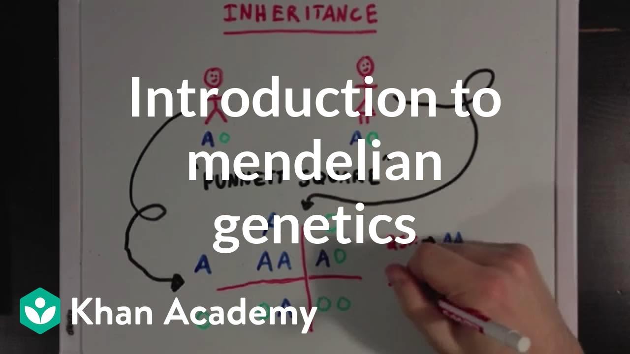
This video provides a concise overview of Mendelian inheritance, clarifying how alleles function as specific variants of genes situated at distinct chromosomal loci. It serves as an essential biological refresher, showing how offspring inherit one allele from each parent to form their diploid genotype, which subsequently dictates their physical phenotype.

---

This lecture provides an in-depth mathematical walkthrough of the product and sum rules of probability. Understanding when to multiply independent probabilities (product rule) versus when to add mutually exclusive probabilities (sum rule) is highly critical, as these identical operations are used to compute expected genotype frequencies in population models.

---

This video provides step-by-step examples of calculating genotype and phenotype outcomes in multi-locus crosses. It reinforces the product rule by decomposing complex crosses into individual, independent single-locus events, preparing you to transition from pedigree-based probability to population-level calculations.

Knowledge Checkpoint

• Define the exact biological distinctions between locus, gene, allele, genotype, and phenotype.
• Determine when to apply the product rule ($P(A \text{ and } B) = P(A) \times P(B)$) versus the sum rule ($P(A \text{ or } B) = P(A) + P(B)$) in genetic scenarios.
• Calculate the probability of producing a specific multi-locus genotype (e.g., $AaBb$) from a cross of two heterozygous parents ($AaBb \times AaBb$) using probability laws rather than a Punnett square.

---

Module 2: The Hardy-Weinberg Principle and Baseline Models

Here, you will transition from individual inheritance patterns to a whole-population baseline model. You will mathematically derive the Hardy-Weinberg equilibrium equation ($p^2 + 2pq + q^2 = 1$), analyze the five core assumptions required for a population to remain in equilibrium, and utilize the Chi-square ($\chi^2$) goodness-of-fit test to evaluate whether real-world population data deviates significantly from null evolutionary expectations.

Recommended Videos

This video fragment summarizes the convergence of Mendelian genetics and Darwinian natural selection, highlighting the algebraic construction of the Hardy-Weinberg equation. By expanding the single-locus, two-allele probability expression $(p + q)^2 = 1$, the video demonstrates how the terms correspond directly to the expected frequencies of homozygous dominant ($p^2$), heterozygous ($2pq$), and homozygous recessive ($q^2$) individuals in a population.

---

This tutorial demonstrates how to approach and solve practical Hardy-Weinberg problems step-by-step. It emphasizes a key methodology: always start by identifying the recessive phenotype frequency ($q^2$) whenever possible, extract the recessive allele frequency ($q$) by taking the square root, and then use the constraint $p + q = 1$ to calculate the remaining allele and genotype frequencies.

---

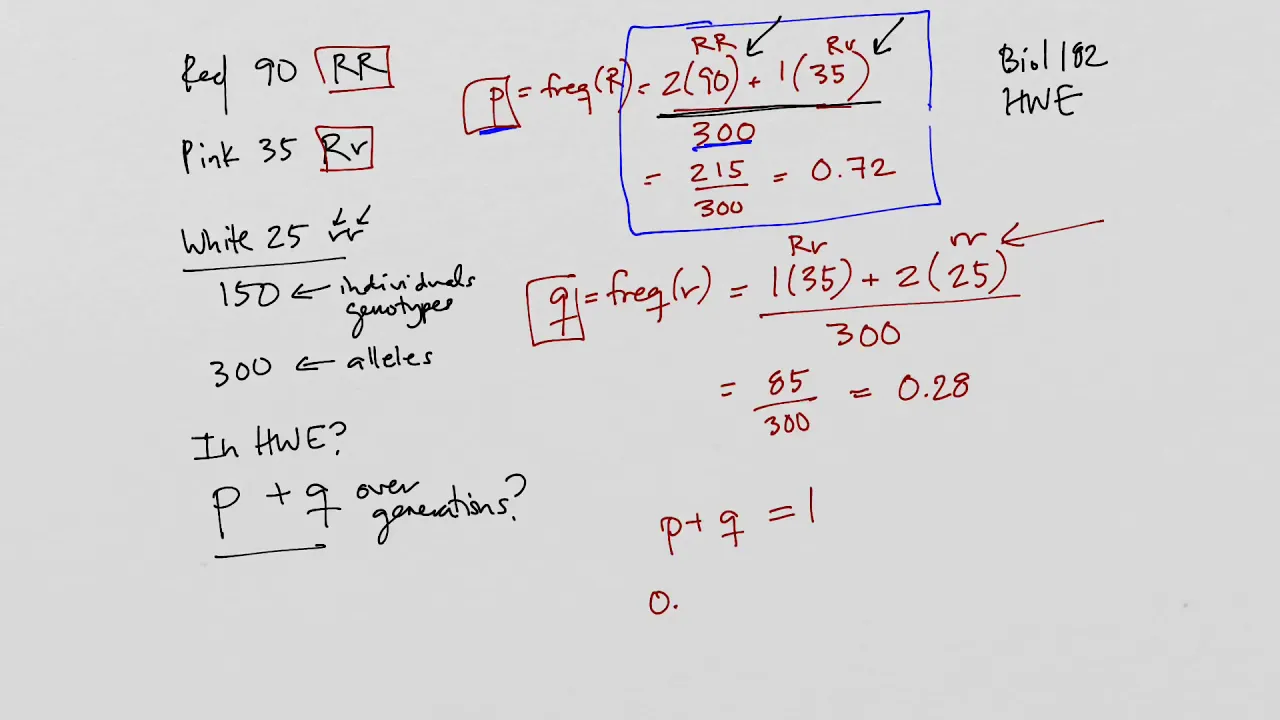
This video walks through how to verify if an active population is in Hardy-Weinberg equilibrium. It demonstrates how to determine actual allele frequencies from observed genotypic counts, calculate expected genotype counts, and perform a formal Chi-square goodness-of-fit test to determine if deviation from equilibrium is statistically significant.

Knowledge Checkpoint

• Derive $p^2 + 2pq + q^2 = 1$ using the probability rules learned in Module 1.
• List the five core assumptions of Hardy-Weinberg equilibrium and explain the physical evolutionary mechanism that occurs when each assumption is violated.
• Given observed counts of three genotypes (e.g., $AA=40$, $Aa=40$, $aa=20$), calculate the actual allele frequencies ($p$ and $q$), construct the expected values under HW equilibrium, and perform a Chi-square goodness-of-fit test (with $df = 1$) to evaluate equilibrium status.

---

Module 3: Mathematical Modeling of Natural Selection

Now we break the "no natural selection" assumption of the Hardy-Weinberg model. In this module, you will learn to model the directional impact of natural selection on allele frequencies over time. You will define relative fitness ($w$) and the selection coefficient ($s$), and understand how different dominance regimes—including complete dominance, codominance, overdominance (heterozygote advantage), and underdominance—influence the rate and direction of allele frequency changes.

Coverage Gap Note: To supplement the following videos, note that the standard mathematical equation for the change in allele frequency over a single generation under selection is: $\Delta p = \frac{p(w_1^* - \bar{w})}{\bar{w}} = \frac{pq[p(w_{11}-w_{12}) + q(w_{12}-w_{22})]}{\bar{w}}$ Where $\bar{w}$ is the mean fitness of the population ($p^2 w_{11} + 2pq w_{12} + q^2 w_{22}$). You are highly encouraged to practice writing out and solving this recurrence equation for different values of $s$.

Recommended Videos

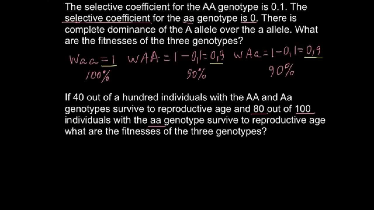
This video clearly explains how to define and relate relative fitness ($w$) and the selection coefficient ($s$). It demonstrates that the most fit genotype in a given environment is assigned $w = 1$, while less fit genotypes are penalized by a factor of $s$ ($w = 1 - s$). This framework allows you to translate raw phenotypic survival data into normalized mathematical terms.

---

This video introduces the calculus-based formulations of selection, showing how the change in mean population fitness over generations is linked to allele frequency change. It derives the fundamental relationship between the rate of change of allele frequencies and the gradient of mean fitness ($d\bar{w}/dp$), bridging classical population models with quantitative evolutionary theory.

---

This rigorous mathematical lecture walks through the analytical derivation of the allele frequency recurrence relation: $p' = p \frac{w_1^*}{\bar{w}}$, where $w_1^*$ represents the marginal fitness of allele $A_1$. By defining the change over one generation as $\Delta p = p' - p$, the lecture provides the essential algebraic steps to track selection dynamics over time.

Knowledge Checkpoint

• If the relative fitnesses of genotypes $AA$, $Aa$, and $aa$ are $1.0$, $1.0$, and $0.8$ respectively, identify the dominance scheme and compute the selection coefficient ($s$) acting against the homozygote recessive genotype.
• Write the mathematical expression for the mean population fitness ($\bar{w}$) in terms of $p$, $q$, and the individual genotype fitness values ($w_{AA}$, $w_{Aa}$, $w_{aa}$).
• Explain why a highly beneficial allele ($s = 0.1$) spreads slowly through a population when it is very rare if it is completely recessive, but spreads rapidly when it is dominant.

---

Module 4: Genetic Drift & The Wright-Fisher Model

This module introduces stochasticity into our evolutionary framework by breaking the "infinite population size" assumption of the Hardy-Weinberg model. You will study genetic drift, the random fluctuation of allele frequencies due to gamete sampling error across finite generations. You will explore the Wright-Fisher model mathematically, which relies on the binomial sampling distribution, and calculate how population size ($N$) determines the probability and rate of allele fixation or loss.

Coverage Gap Note: Because YouTube videos on the formal matrix algebra of Markov chains in Wright-Fisher models are scarce, remember the key mathematical relationship: the variance in allele frequency due to drift after one generation is: $\sigma^2 = \frac{p(1-p)}{2N}$ For a neutral allele, the probability of eventual fixation is equal to its current frequency ($p$), and the average time to fixation for a newly arisen neutral mutation is $4N$ generations.

Recommended Videos

This video delivers the mathematical scaffolding for modeling genetic drift using matrix algebra and the Wright-Fisher framework. It details the core model assumptions—finite population size, infinite gametic pool, random mating, and non-overlapping generations—and demonstrates how allele frequency transitions can be treated as a Markov chain.

---

While this is a statistical modeling lecture, this selected clip focuses on the binomial sampling formula. It explains how to calculate the probability of observing a specific count of outcomes given an underlying probability $p$. This exact mathematical mechanism forms the sampling foundation of the Wright-Fisher model, where the next generation's alleles are sampled binomially from the current generation.

---

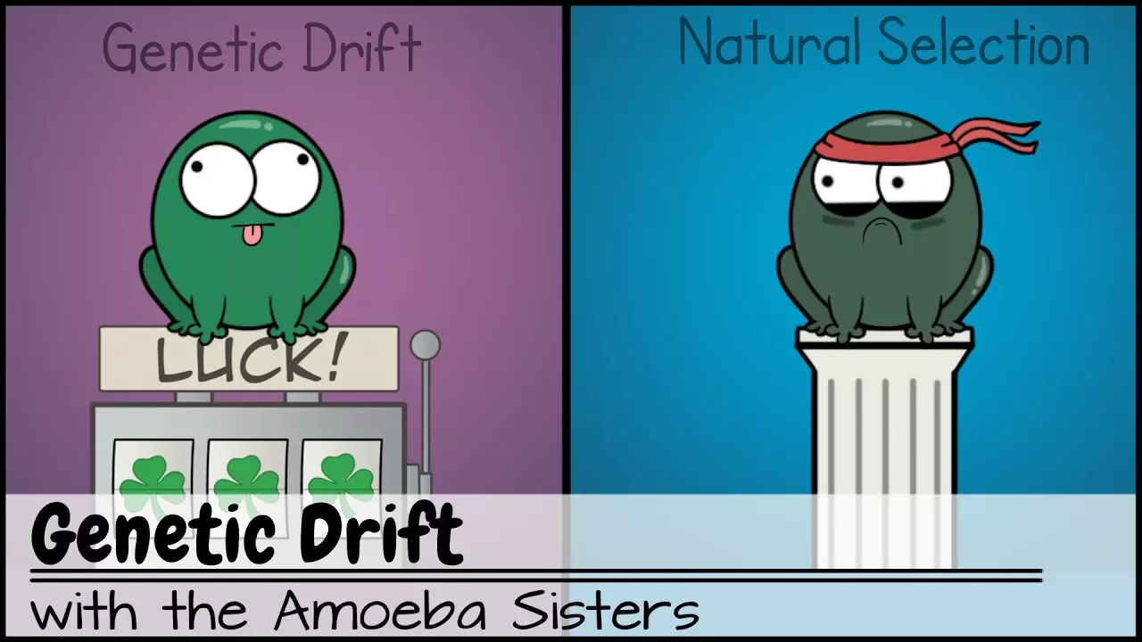
This video provides an accessible, visual exploration of genetic drift, detailing its physical manifestations such as the bottleneck effect and the founder effect. It contrasts drift's non-directional, stochastic nature with the directional sorting of natural selection, serving as a conceptual anchor for the underlying mathematics.

Knowledge Checkpoint

• Explain how binomial sampling is used in the Wright-Fisher model to calculate the probability of an allele frequency shifting from $i/(2N)$ to $j/(2N)$ in a single generation.
• Calculate the variance in allele frequency after one generation due to drift for a diploid population size of $N=50$ and an initial allele frequency of $p=0.5$. Contrast this with $N=5000$.
• If a neutral mutation occurs at a single locus in a diploid population of $100$ individuals, what is the exact probability that this new mutation will eventually reach fixation in the population?

---

Module 5: Gene Flow, Mutation, and Joint Forces

In this module, you will incorporate the final major microevolutionary forces: mutation and gene flow (migration). You will study how recurrent mutations alter allele frequencies and derive the mathematical equilibrium of mutation-selection balance. Additionally, you will look at how migration introduces alleles into a population, acting as a homogenizing force that counters local selection and genetic drift.

Coverage Gap Note: While reviewing these materials, write down and memorize these two core equations:

1. Mutation-Selection Balance: For a completely recessive deleterious allele with mutation rate $\mu$ and selection coefficient $s$: $\hat{q} \approx \sqrt{\frac{\mu}{s}}$
2. Continent-Island Migration Model: The change in allele frequency on the island ($\Delta p$) per generation is: $\Delta p = m(p_m - p)$ where $m$ is the migration rate and $p_m$ is the allele frequency of migrating individuals from the mainland.

Recommended Videos

This video presents the mathematical derivation of mutation-selection balance. It explains how deleterious recessive mutations are introduced into a population at rate $\mu$ and eliminated by selection at rate $s$, and shows how these opposing forces reach a stable equilibrium ($\hat{q} \approx \sqrt{\mu/s}$).

---

This short segment from an MIT lecture highlights how population-level genetic variation is a dynamic balance of multiple simultaneous evolutionary forces. It introduces forward and reverse mutation rates ($f$ and $r$) alongside selection parameters, highlighting how populations rarely experience just one evolutionary force in isolation.

---

This video defines migration (gene flow) in population genetics as the physical movement of individuals and their alleles between populations. It explains how gene flow acts to homogenize genetic differences between distinct geographic groups while introducing novel variation locally.

Knowledge Checkpoint

• Calculate the equilibrium frequency ($\hat{q}$) of a lethal recessive allele ($s=1$) if the mutation rate ($\mu$) generating it is $10^{-5}$ per generation.
• Using the continent-island model, if the island allele frequency is $p = 0.2$, the mainland frequency is $p_m = 0.8$, and the migration rate is $m = 0.1$, calculate the island allele frequency in the next generation ($p'$).
• Describe how gene flow and genetic drift act as opposing forces on genetic differentiation between populations.

---

Module 6: Computational Simulations in Population Genetics

In this concluding module, you will translate the mathematical models from modules 1-5 into interactive computational tools. You will explore how to simulate genetic drift and selection using software modeling packages, learn to interpret demographic trajectories, and study how spreadsheet and programmatic frameworks can run thousands of genetic iterations to visualize long-term evolutionary outcomes.

Recommended Videos

This video demonstrates how to set up and run population genetics models using an Excel-based spreadsheet simulator (DE 1.0). It showcases how you can manipulate populations by adjusting parameters for population size, selection coefficients, migration rates, mutation rates, and initial allele frequencies to observe stochastic or deterministic trajectories.

---

This video introduces a programmatic approach to evolutionary simulation using Python. It shows how to represent organisms as objects containing traits like speed and position, setting up loops where survival and reproduction are dictated by their genetic values. This provides a template for translating abstract selection math into functional computer code.

---

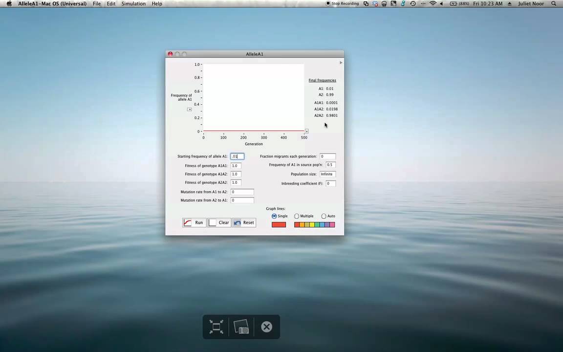
This walkthrough explains how to use the AlleleA1 software simulation engine. It shows how the program calculates allele frequency trajectories over hundreds of generations by simulating the joint effects of finite population size, mutation rates, migration, and genotype fitness values.

Knowledge Checkpoint

• Explain how you would structure a Python loop or an Excel spreadsheet to calculate and log the allele frequency $p$ over 100 generations under directional natural selection.
• In a simulation program like AlleleA1, if you set the population size $N$ to be small (e.g., $N=20$) and selection coefficient $s = 0.2$ in favor of allele $A$, describe how the trajectory of $p$ would look compared to running the same parameters with $N=10,000$.
• Design a simple pseudocode algorithm that simulates genetic drift using a random number generator and a binomial sampling function.

---

Course Map

Below is the recommended learning pathway. Ensure you complete the prerequisites in the earlier modules before tackling modules 5 and 6, which represent the integration of all mathematical evolutionary forces.

---

Key People Index

• Gregor Mendel: The Augustinian friar who established the laws of segregation and independent assortment, demonstrating that traits are inherited in discrete particle-like units (alleles) rather than through fluid blending.
• G.H. Hardy & Wilhelm Weinberg: The English mathematician and German physician who independently formulated the null algebraic baseline model ($p^2 + 2pq + q^2 = 1$) to describe allele frequencies in non-evolving populations.
• Ronald Fisher & Sewall Wright: Key foundational theorists of population genetics. Fisher developed models focusing heavily on selection in massive populations, while Wright introduced key models of genetic drift (including the Wright-Fisher model) and migration.
• Richard McElreath: Evolutionary anthropologist and statistician whose lectures on Bayesian methods highlight binomial sampling, the foundational probability architecture used to track stochastic allele transitions.

---

Final Self-Assessment

Complete this final checklist after finishing all modules to verify your mastery of mathematical population genetics:

• Explain how to derive the Hardy-Weinberg equation using the sum and product rules of probability.
• Determine when a population deviates from Hardy-Weinberg equilibrium using a Chi-square test, and state the degree of freedom used for a bi-allelic locus.
• Compute the mean population fitness ($\bar{w}$) for a population with allele frequencies $p = 0.6, q = 0.4$ and genotype fitnesses $w_{AA}=1.0$, $w_{Aa}=0.9$, and $w_{aa}=0.2$.
• Compute the shift in allele frequency ($\Delta p$) over one generation under selection using the standard recurrence relation.
• State the definition of the selection coefficient ($s$) and detail how it relates to relative fitness ($w$).
• Calculate the variance in allele frequency due to genetic drift across one generation in a diploid population of size $N$.
• Explain how the Wright-Fisher model uses a binomial distribution to calculate transition probabilities for allele frequencies.
• Solve for the equilibrium allele frequency ($\hat{q}$) under mutation-selection balance for a deleterious recessive mutation.
• Solve for the next generation's allele frequency on an island after accounting for mainland migrants.
• Contrast how population size ($N$) influences the relative power of genetic drift versus natural selection in determining the fate of an allele.
• Write down the conceptual pseudocode required to run a 1,000-generation simulation modeling both genetic drift and selection simultaneously.