











![[BayesCog] SoSe 2021 Lecture 06 - Linking model and data](https://i.ytimg.com/vi/xEmDDwCF9-Y/hqdefault.jpg?sqp=-oaymwEmCOADEOgC8quKqQMa8AEB-AH-E4ACoAuKAgwIABABGBMgTSh_MA8=&rs=AOn4CLCTPZBMPdlbUNwaIgavQTT3XEOLLA)


![[PHYS574] 6. Markov Chain Monte Carlo](https://i.ytimg.com/vi/TOTWOvszFnA/maxresdefault.jpg)
![[Коллоквиум]: Вероятностное программирование](https://i.ytimg.com/vi/ZHERrzVDTiU/maxresdefault.jpg)






Bayesian inference is a logical approach to statistical analysis where for each possible explanation of the data, we count all the ways that data could have occurred, and explanations with more ways to produce the data are considered more plausible; this counting process is implemented through methods like grid approximation and posterior predictive distributions to make inferences about parameters such as the proportion of Earth's surface covered in water.
Bayesian Inference | Statistical Rethinking 2022 Lecture 02
Added:Fundamental probability theory, specifically conditional probability and the mathematical formulation of Bayes' Theorem.
The basic concept of probability distributions (both discrete and continuous), including probability density functions (PDFs).
Basic programming literacy in R or Python to comprehend the computational implementation of grid approximation.
The conceptual distinction between parameters (unobserved variables to be estimated) and data (observed outcomes).
Markov Chain Monte Carlo (MCMC) sampling methods, which are necessary when grid approximation becomes computationally intractable in higher dimensions.
Bayesian linear regression and the formulation of generalized linear models (GLMs) using probabilistic programming tools like Stan or PyMC.
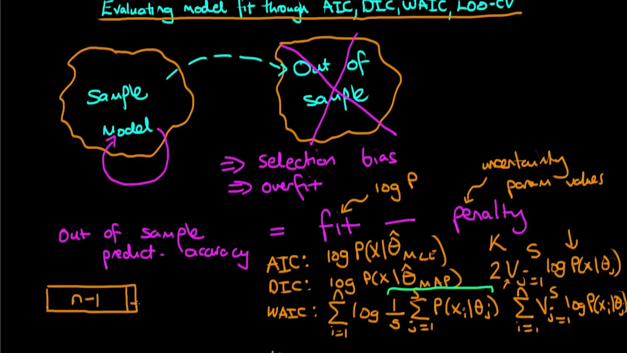
Model evaluation and comparison techniques, such as Information Criteria (WAIC) and Leave-One-Out Cross-Validation (LOO-CV).
Constructing and interpreting multilevel (hierarchical) models to account for structured, nested, or grouped data.
92.8K views0likes1:12:46Original Release: 2022-01-04
welcome to the second lecture in statistical rethinking 2022. we have a lot of work to do today we're going to start with some small problems in bayesian inference and then we'll use the same logic from these problems throughout the rest of the course first small problem is the earth when you consider the earth from space it is mostly water two-thirds is covered in clouds on average and about 70 percent of the surface is covered in water how would you know that well we know it because we have high quality maps but you can also imagine a randomized monte carlo process to learn it if you imagine all the space debris crashing into the earth little rocks meteors all the time about 70 percent of them land in water and about 30 on land so if you could catalog those impacts you would have a data set you could use to make inferences we can't do that we're not in orbit we're not going to hurl rocks at the earth and count the impacts but we could take an inflatable globe and do this when i've taught this course in person this is exactly what i've done i have an inflatable globe in my office that i use for this purpose you can throw it into the audience and then when a person catches it they look where their right index finger is pointed and if it's water we record a water and if it's land we record a land after a certain number of samples we have a data set and now the question is what do we do with that data set so let's imagine how that process looks here's a virtualized version of my inflatable globe it's a geographically accurate more or less computer version of the globe and we can spin it and take a random sample first one is land the second is water third is land fourth is land fifth is water sixth is also water seventh is water eighth is land ninth is water and the tenth is water and we'll stop there now we have a little modest data set ten samples from our globe these are random samples from the surface of the earth how should we use the sample to make an inference about the proportion of the earth's surface that's covered in water there are lots of ways you can use data to produce summaries and we have to have an answer to to this also given a summary how would you represent uncertainty obviously more data is better with only five samples from the globe we would have less certainty than we do with our 10 and if we had 20 or 40 or 80 or 160 it would be even better how should we represent that uncertainty we're going to use bayesian data analysis to answer all three of those questions at once bayesian data analysis is a very modest approach to inference and it can be summed up with the words on this slide for each possible explanation of the data we're going to count all the ways the data could happen and those explanations with more ways to produce the data are more plausible now i'm going to spend the rest of this lecture expanding on this and making it algorithmic so you can understand how it works but you should know that every bayesian model instantiates this approach and this is how data are used to produce inferences how they are summarized and how uncertainty is represented is all through counting of ways that data can happen okay so we're going to apply that logic to our proportion of the earth that's covered in water problem this is a bit too complicated a problem to start with though because there are an infinite number of explanations because each proportion whether it's 0.1 or 0.2 or 0.5 is a possible explanation of the data as you'll see and they're an infinite number of those proportions right because they're an infinite number of real numbers between 0 and 1. so let's start with something a little easier and where we can really just count a finite number of explanations and then we'll loop back to the earth problem this particular picture of the earth is a famous one it's called the blue marble it was a photograph that was taken from one of the apollo missions maybe apollo 17 in the 1970s um let's shrink this blue marble down and we're going to think about marbles in a bag as an initial analogy for how we do inference in these settings so now imagine there's a bag represented on the slide on the left and it's going to contain four marbles and some of them are blue like the earth and some of them are white and but they're only four and we take this as given information but you don't know how many of the marbles are blue and how many are white but with this information we can enumerate all the possible explanations of any sample you get and those explanations are just the contents of the bag and there are five different possibilities shown here in the middle column first all of the marbles could be white second one could be blue and three could be white two could be blue and two could be white three could be blue and one could be white or finally all four of them can be blue we're going to assume that we've reached into the bag and sampled with replacement three marbles so what that means to sample with replacement is after we draw out a marble we put it back we shake the bag we draw another we've done that three times and we've observed in sequence blue white blue as our sample and now the question is given that observation how can we use that to make an inference about which of the possible contents are most likely and we're going to do it the base way just by taking each possible explanation and counting all the ways that the observations could arise given that assumption given that explanation so in this case let's take the second one to start the second possible set of contents one blue marble and three white marbles and we're going to assume the bag contains that for the moment and that by assume here we just mean we're going to playfully uh assume that's the case that that's the reality we're in and we're going to deduce the consequences of that assumption but i assume i don't mean we're going to assume it's true forever for now this is a form of analysis for the moment we assume it's true as you'll see we'll do the same for all of the possible explanations so how many ways are there to observe blue white blue if the bag contains one blue and three white marbles we're going to use a device i call the garden of forking data and in the garden of forking data what we do is we draw out all the possible events that could happen from each sample so imagine our first draw from the bag this is our first possible observation there are four things that could happen assuming the bag contains one blue and three white marbles so there in a sense in the garden of forking data there are four possible paths drawn here on the screen and then we considered the second possibility the second draw from the bag we get another marble and there are four possibilities for that as well the same four possibilities but those branch off from the previous four possibilities because these give us different data sets different samples depending upon what happened in the past and what happens on the second possibility so there were four possibilities on the first draw and there are four plus 4 plus 4 plus 4 or 16 possibilities on the second draw so 16 possible different data sets at this point and then the third and final draw in this example the third possible draw from the bag again whatever happened on the first and second draft to give us each of those 16 data sets possible data sets each of those has four additional paths drawn from it same four one blue and three white marbles and for a total of 64 different possible data sets and three draws from the back okay why have we done this we're doing this because now we have a device a visual device that lets us count up all the ways that any particular data set could arise assuming the contents of the bag are one blue marble and three white marbles again we're going to look at the other possibilities next but we're going to stick with this one for now so let's trace that out let's imagine our first observation and that's a blue marble at the bottom of the slide and there's exactly one path by which that can happen highlighted here in red so there's one way for that first observation to happen assuming or conditioning on uh that the true contents of the bag are one blue and three bite marbles and now the second observation is a white marble shown at the bottom how many ways could that happen there are three uh branching off from the first possibility the all the possibilities on the on the right hand side of this garden of forking data have already been foreclosed have already been forbidden by the fact that the first observation was blue so the second one is white and there are three paths now by which this data set could arise and then we consider the third and final observation this is blue and so we trace the blue paths that originate from the three uh valid paths that we had so far so there are three total ways for the sample to arise assuming the bag contains one blue and three white marbles so let's summarize that because this is our goal actually in bayesian inference is to get this information to count up the number of ways to see the sample if the bag contains in this case one blue and three white marbles or more abstractly we want to count up all the ways the data could arise assuming for each explanation assuming some explanation were true just playfully for the moment we count up all the ways that the data could arise given that explanation and then we're going to compare the different explanations based upon these counts and that is bayesian inference although it's usually presented in a fancier way so let's put that into our our table of results now we come back to our table from the earlier slide summarize the garden of forking data in the second explanation there's one blue and three white marbles there are three ways to realize the sample we have with that let's consider the other possibilities now we get the first one pretty much for free it's forbidden by logic the bag cannot possibly contain all white marbles because we have seen a blue marble we have seen two of them in fact well they could be the same blue marble likewise the fifth explanation all blue marbles is also forbidden by logic because we have seen a white marble but what about the other two possibility three and possibility four with two and three blue marbles respectively let's take those in turn so consider the third explanation two blue marbles two white marbles let's draw the guard two blue marbles at the bottom two white marbles and then from each of those branching off again two blue two white and now we trace out all the ways the sample could happen so from the bottom we sample a blue there's two ways for that to happen from each of those we sample a white there are two ways each for that to happen so now four in the middle uh row of the garden and then for each of those we draw a blue marble and there are two ways for that to happen again and so we end up with eight possible paths i'll give you a moment to trace this with your eyes and count it out you see that there are eight valid paths consistent with the sample of blue white blue now the fourth possibility three blue marbles and one white marble same exercise gonna draw the garden and trace the pass three blue marbles one white to start and then from each of those again three and one and then three and one and now three ways to get a blue one way for each of those to get a white and then three ways to get a blue from each of those for a total of one two three four five six seven eight nine valid paths ways to realize the data assuming the bag contains three blue and one white so let's summarize now put all the numbers in the table the first explanation is forbidden because if the bag didn't contain any blue marbles we wouldn't have seen any so there are zero ways uh for that explanation explanation number one here to explain the data and the second one this is the one we started with there are three ways and then eight and then nine and then again five forbidden by logic because we have seen a white marble so these are relative numbers these are numbers of ways for each explanation to produce the data we've seen and this is basically it in bayesian inference real data analysis problems well this is a this is a real data analysis problems the typical let's say typical data analysis problems in the sciences and in basic research look a lot fancier than this and these calculations are often automated for you but this is the logic of probability theory here is we count up all the ways the data can occur and then we use across a range of explanations and then we use those counts to compare the plausibility of the different explanations so let's try to summarize that now let's let's make this feel a little bit more like probability theory it's what i call the unglamorous basis of applied probability things that can happen more ways are more plausible and that's pretty much it why do we do this because it's unreasonably effective that's why and it's nothing more than logic we state our assumptions those assumptions have implications for the data for for the observations and then if assumptions that are more compatible with observations are considered more plausible so summarizing at the bottom we have all the possible compositions of the bag these are explanations for the observations emerging from the bag each of those we could assign some index what we call a parameter here p which is just a proportion of blue marbles in the back this is not necessary but this is the more conventional way we talk about these and this will help us relate it to the coverage of water on the earth example which we're going to return to shortly so the proportion of the bag that contains blue the proportion of the bag that is blue marbles ranges from zero to one and the possible explanations are zero point two five point five point seven five or one for each of those possible explanations we deduced that there are zero three eight nine zero ways respectively for each of those explanations to explain the data and then finally these ways are are meaningful only to the extent that they are different relatively different from one another the absolute counts are not wanted but it's important all of them could be small all of them could be large what matters is there are the relative values and so what we do to deal with differences in the sizes of data sets and and the arbitrary combinatorics of particular problems is we normalize these counts so that they all sum to one and that's all i've done here is taken uh the sum of the ways to produce data column the 3 plus 8 plus 9 and divided each of those numbers by that here i can show you in code what that means we just make a vector in r called ways which contains the numbers 3 8 9 and then i divide that by the sum of the vector and that gives us the number shown on the right hand column of the table the plausibility column these are 0.15.4 0.45 these are these are probabilities i'm calling them plausibilities because that's their function and inference but this is all probabilities are as well and so the code snippets i'm going to show in in the lectures are all our code but uh as i'll remind you a little bit later in this lecture the almost all the code examples in the book and the course have been translated to other major languages like python and julia so if you look at the course web page you can plug into the your preferred scripting environment okay this procedure can handle the data all at once or as it comes in and that's a great feature of bayesian inference is there's this thing called bayesian updating that is when new data arrives we don't we don't have to redo the whole calculation we can just take the old answer and update so let me show you the logic of that and uh actually surreptitiously here we're deriving a law of probability the the product law so we get one more draw from the bag the blue marble remember our five conjectures our five possible explanations for the contents of the bag for this new sample that we've just seen a blue marble it's very easy to count up the number of ways each of these conjectures could explain it if if the bag is all white marbles there will be zero if there's one blue marble it'll be one and if there's two there's two if there's three there's three if there's four there's four right hopefully that's obvious and then we have our previous counts zero three eight and nine from the sample of three that we had before instead of redrawing the whole garden and doing this over again we can just multiply these numbers together actually why because remember in the garden at each additional step each additional ring in the garden that grew you were multiplying the number of steps it went from 4 to 8 to 64 as you branched out and that was because they were multiplying so if events happened independent in this the proper way to count all the possibilities is just to multiply the counts together right so think about it this way if there's two things if there's two ways for one thing to happen and two ways for some independent thing to happen then then there are two times two or four ways for both events to happen together and that's all we're doing so we multiply obviously zero times zero is still zero uh three times one is three eight times two is sixteen 9 times 3 is 27 and 0 times 4 is 0. so now our our counts are 3 16 and 27.
the three blue marbles is looking more and more plausible here more and more likely but again it's the relative values here the relative numbers of ways that matter not their absolute counts in any reason besides data set if you did this manual kind of counting the numbers would get really astronomical really very fast because of the way combinatorics work and so that's another reason we must normalize at each step by by summing and dividing each by the sum okay let me try to do some summary here what are the rules in bayesian updating what you must do is state some causal model some mechanistic model for how the observations arise uh given each possible explanation now we might we don't know the true explanation but you have to know enough about or believe enough about the mechanisms of each explanation that you can state what the data sets that would emerge from it look like second you count the ways the data could arise for each explanation using the assumptions you made in in step one and then three relative plausibility uh is the relative value from two and what do we do with these relative plausibilities well lots of things they're used for inference and we'll see lots of examples of that going forward but you'll see as we turn back to the water on the earth example you'll get a sense of what it does what these the information contained in these relative possibilities but they tell us in a crude sense which explanations are plausible and which ones are much more or or much less plausible than others okay so let's go back to the globe now and we're going to repeat all that counting but now for an infinite number of possible explanations y infinite because they're an infinite number of proportions between 0 and 1 and we want to rank them all or nearly all of them so for each possible proportion of water we're going to count the number of ways the data could happen and this requires us as always to state how the observations are generated and that's how are they generated well by tossing the globe around not by throwing meteors at the earth and counting splashes right so let's let's imagine that let's imagine here i've virtualized the globe tossing exercise in the computer and we're going to take a first toss from the virtual globe and that'll happen on the left here and on the right i'm going to draw a graph of the relative plausibilities of each proportion so if you look at the graph on the right the horizontal axis is all the possible proportions of water from zero to one it's a proportion of water on the globe and the vertical axis is this thing called density which i'll explain in a moment and the the dashed line that you see at one this is the information we have before we see any data we'll talk more about that in a moment so we start and we get a first sample and it's land and the implications of that according to counting all the ways is this diagonal line starting at its maximum on the far left at zero proportion of water and going down to one so i'm gonna pause for a second and talk a lot about this one particular slide and i'll move more quickly through the slides that follow because they have the same structure but we need to get this right to begin now so this this dashed line that i mentioned before is typically called the prior that that was what we knew about the relative plausibilities of each possible explanation before the data arrived and this this red or or pinkish diagonal line is called the posterior and that is the relative plausibilities of each possible explanation after the data arrive and the observation in this case is just one land sample right so why does the posterior have this shape well i'm going to talk about this on multiple slides to come and i'll say it now too it's just the relative numbers of ways to observe a land sample given each possible portion of water so think about it for a second so on the far left if the earth had no water on it at all the value on the horizontal axis was zero then that would be the maximum number of ways that is all the ways to observe land you would always observe land and then as the proportion of water increases as we move to the right on the graph the relative number of ways to observe land decreases and it decreases in a linear fashion because that's how proportions work until you reach one on the far right and then it would be impossible to observe land and so that is where it reaches zero because there are zero ways to observe land if the proportion of water in the earth is one and so it has gone to zero at that point so there is nothing about the shape of this posterior distribution here that is anything but logical it emerges purely logically from our assumptions there's no choice about it after the description of how the globe tossing exercise works everything else is deduction from that point on okay final thing to say about this slide is density this weird word density density is a particular concept in probability theory and we're going to talk about it multiple times in the course for now it's sufficient to understand it as relative plausibility of the proportion of water and its relative value and the actual numbers uh don't focus too much on them right now we're going to talk about this more in in the weeks to come because sometimes it does matter but for now it's fine to to have a heuristic understanding of this as relative plausibility okay now let's take a second toss from the globe so i'll repeat the first one and now a second one and we get water and now here's the updated posterior distribution and i've left the prior distribution from the previous sample that is just one land on there for comparison so you can see in each step of the animation what has changed by adding one more data point as it were so let's focus on on this shape this little dome for a second and ask why it needs to look like this it has to look like this because of well logic because bayesian inference is just logic but there's no it's no accident that it looks exactly like this so it just comes from multiplying two diagonal lines together so let's let's start in this slide on the on the far left here and look at these there's a pink line and a blue line the pink line is the relative plausibility of of a single land sample for each possible proportion of water that's the graph on the far left the relative possibility of land across all the proportions of water on the horizontal and then in the middle of this slide we have the same construct but for a water observation a single water observation it's still linear but it's just flipped because now we're talking about the other possible event along the proportion of water on the globe that is it's maximized at one and it's zero at proportion of water of zero and remember in the in the garden of forking data when you get independent observations and you want to update you multiply the plausibilities or the numbers of ways together and so we can literally multiply these two curves together and that's how we do it what does that mean that means for each possible proportion of water on the horizontal axis here i've drawn these vertical dashed lines to give you a visual guide to what i'm going to say we find those matching values and we multiply them together and then we put the product the result on the graph on the on the far right and this is our new posterior distribution so you can imagine starting on the far left and tracing out that multiplication and it will increase until the midpoint and at the midpoint it's maximized because there's no low values both lines are at the same value here and there's no implausible observations to drag the whole curve down but this must be symmetric because the lines are symmetric and so as we continue on to the right it goes back down to zero why because at a proportion of water 1 it would be impossible to observe land and so that cancels the curve essentially i hope this makes some sense i'm going to stick with this logic for a little bit longer what i want you to get from this is that the shape of these curves uh comes entirely from the implications of how the proportion of water relates to to the probability of seeing a land or a water that is those diagonal lines are our mechanistic assumptions about how the sampling works and then all bayesian updating is is multiplying a series of these diagonal lines together to get some curve but the number of possible curves that can arise from that is really huge depending upon the exact sample you get so let's move towards that and give you some appreciation for it oh a little bit of drawing the owl if you don't mind if you want to mechanistically play with this just convince yourself in r this one line at the top plot 0 to 10 times 10 to 0 will give you the shape the exact shape of that posterior distribution seen here okay now we get a third toss from the globe so again here's the first one and the second and the third another land and so now we've got land water land and we've got this particular curve which does not maybe look to your intuition like it merely emerges from multiplying diagonal lines together but it does it comes from multiplying these three diagonal lines the land water land line so it shifted more towards land to the left half of the graph because we have twice as much evidence for land as we do for water at this moment but notice that basically all all the proportions of water are still in play because we have so very little data and now you can start to appreciate how relative plausibility works as we get more and more evidence this this curve is going to get and more concentrated in particular region of the horizontal axis and that's how the inference works and we get more confidence so again a little bit of drawing the owl if here's a one line of our code that will draw a plot which has the same shape exact shape as this posterior distribution you're just multiplying these vectors together ten to zero and then zero to ten for a water observation and then another ten to zero for land and those are those diagonal lines okay now let's do 10 samples and i'm just going to animate the whole thing through here so you can get an idea how this works and you can back up the video a bit and watch this over and over again if you like and develop some intuition for what's going on i think you'll see all these principles are applied and each time we get another sample we just multiply another diagonal line whether it's for land or for water and that adjusts the curve so you'll see when it's a water sample the curve shifts to the right like there and when it's a land sample it'll shift to the left if we get it yeah there we go land sample and then back again notice that the curve is also getting narrower and taller and that's because the the total plausibility is is fixed in in this distribution because the distribution always sums to one that's it sums the one because we make it do that that's that normalization step uh and so the area under the curve is fixed to be one that's what makes it a probability distribution and so as it gets more concentrated it has to get taller otherwise its volume wouldn't be the same or that's volume it's area right the area under the curve so this is a sense in which more and more evidence leads to a smaller range of values on the horizontal axis being plausible and you have greater and greater confidence that's a nasty word i don't like to use that more and more plausibility is bunched up on a smaller number of values okay so let's let's think about this a little bit more animated we start out with this sort of no information state shown in the upper left here of having no idea at all how much water is covered is how much of the earth is covered by water after one sample we get this diagonal line then we sample a water and now there's essentially two of these diagonal lines put together and it's symmetric evidence and after a third and after fourth and after a fifth and after a sixth and after a seventh and after an eighth and what i want you to realize about this whole procedure is that we've done it step by step one sample at a time but of course you could take the whole sample and do it simultaneously as one big updating moment go straight from the flat prior in the upper left to the curve in the lower right if you just gave the machine all the data at once and that's how we usually do data analysis but you can do it step by step like this and that's why it's called bayesian updating because there's an implied series of updates as the golem the little machine has has learned things it thinks it's learned things from the data using the assumptions you've programmed it with so this is sort of the world's most basic example of bayesian inference but it has all the general features so i want to spend a few slides now just talking about those general features and they may be in conflict with your previous statistics education and that's why i want to call some things out so the first thing to notice is there's no minimum sample size in this business there's no such thing one data point's enough in fact zero data points is a sufficient sample size to do analysis and we'll we'll do a lot of analysis in this course with zero data because that's how we understand what the model thinks before it sees any data at all that's how we explore the implications of the model before we add evidence that's what something we'll call prior predictive simulation i'll show you an example near the end of this lecture but usually we want some data if you have one data point it's already worth updating possibly and of course as you see here like the example on the slide you don't learn a lot from one sample because most explanations are still in play so your beliefs don't change a lot but there's no sense in which there's some minimal sample size required for inference the relative plausibilities tell you here that very little can be concluded you haven't learned much second the whole shape of the posterior distribution the blue curve on the slide it essentially embodies the sample size so in in other statistical frameworks sample size it has some kind of magical quality you're always reporting it and talking about it and you need to use it to calculate things called degrees of freedom and and so on sample size has no comparable role in bayesian analysis because all the information that is relevant to inference about the explanations has already gone into constructing this curve and so if you get new data or for anything you'd like to to know about the explanations is already embodied in the curve and if you get new data you don't need to redo those calculations you can just start with the curve you have and go forward doing updates one thing you'll help you get an intuition though is of course sample size matters and as you get more and more data the curve gets narrower and taller uh third point estimates don't really have a big role in bayesian inference because the estimate is the curve what do i mean by this so given any particular posterior distribution like the the dash gray one on this slide you can pick a lot of reference points so you could take the point at where it's maximized for example the mode and say that that's your best estimate if you like you could also take the mean and which of these is is the best summary of the curve depends actually upon a lot of sort of extra scientific criteria like the costs and benefits of different different actions that you take using this information and those are not usually uh criteria that we have strong feelings about in basic research but you may very well in industry and if you want to read more about this in chapter three of the book i talk about how utility functions that is explicit assumptions about costs and benefits can be used to decide which point estimate you might want to use but in general in scientific publications there is no valid point estimate the distribution is the estimate and we want to report the whole distribution to a useful level of accuracy and when you do anything with the model as you'll see again and again in this course and like produce predictions or report causal effects compute counterfactuals anything at all you always use the entire distribution there is no case in which you take a a summary of the posterior and then do subsequent calculations with it or as i like to say summary is always the last step all calculations and and machinations with a bayesian model must use the entire posterior distribution all the time otherwise you're throwing away uncertainty and you'll get overconfident answers okay fourth thing i want to say is intervals also don't have a really strong role to play in bayesian inference there i summarize this at the top of the slide by saying there is no one true interval but you can report any interval you want all they're doing is communicating the shape of the posterior distribution so there's an infinite number of intervals that you could draw and they're all arbitrary they just have different utility given the communication function you have in mind so you could draw a 50 interval for example this interval i've drawn here is the middle 50 percent uh middle 50 percent of the quantiles of of the probability mass so it captures a central range but there's actually an infinite number of 50 intervals because you could slide this interval left and right and still capture 50 of the mass so this the fact that this is central it's heuristic and it seems reasonable but there's no strong logical reason that you would have to use this at all and the same is true for any other width of interval we could make something bigger like 89 i'm quite fond of 89 intervals i use them in the book i use them in the course and i use them in my papers um uh but again it's just an arbitrary number it covers a very wide range of the most plausible values and it's it's a convenient summary sometimes but there's nothing special about it there's nothing special about it because nothing nothing special happens at the boundary at the edges of these intervals there's no it's just a continuous reduction in plausibility as you leave the interval there's no special cliff that anything really falls off of even though it looks like there's a cliff at the end of the interval we could use really wide intervals sometimes these this is the right thing to do because you want to make some argument about really all of the plausibility is in is in some range and so you can use 99 percent or even 99.9 percent intervals to report that range conventional 95 intervals that you see quite often in scientific publications this is an obvious superstition and what do i mean by that people sometimes endowed the 95 interval with with seemingly magical powers as if uh this was the only interval you needed to report and if um some particular value like zero is contained in that interval then that means there's no effect and none of this is logical uh it's purely conventional but people and people know that uh if you push anybody a little bit they'll admit yeah of course it's a convention but we're humans and we live kind of in a prison of conventions right that's the way culture works so it's hard to break free from these things but i think we can break some of that spell by just stating publicly look this is a superstition there's nothing logical or mathematical about some particular 95 interval this is especially true in bays because we're not using these intervals to do error control that's not what we do with them there's nothing about type 1 error here or so on that now i should i want to say that it doesn't mean base doesn't do error control of course it does because it finds the most plausible values and helps you avoid mistakes but the intervals don't have that function they're not calibrated to do that all right keep saying nothing magical happens at the boundaries yeah so uh one last slide before we take a little bit of a break here we all need a bit of a break um that's a an installment i want to call letters from my reviewers so i like all of you i write papers and i put stats in there and one of the questions i often get when i teach is how do you when you put bays in your papers how do you deal with reviewers who are ignorant about bays and say silly things and i always say well you you try to educate them and remember that you're talking to the editor not to the reviewer but the comments that reviewers write are often quite overconfident uh when they're ignorant of bays because they'll project their ignorance on to me because they don't know who i am i'm just some anthropologist right and that's fair i mean i don't want uh i don't want any any um special treatment from reviewers uh but here's here's one that that i collected that i think is quite telling about the kind of latent assumptions that come from other statistical frameworks so the this one reviewer said uh this was last year in 2021 the author uses these cute 89 intervals i do i'm guilty but we need to see the 95 percent intervals so we can tell whether any of the effects are robust so they they were the reviewer was saying that i needed to add conventional 95 intervals and the the implication here is they were going to see if zero was contained in any of those intervals and if so they would declare the effects not robust now none there is no statistical framework in which this program is legitimate but you see these things in reviews my response of course is that look the this is bays and we're not doing air control with the intervals significance tests here are illegitimate um the width of the intervals is irrelevant and all of the prediction curves and everything else contained in the paper uses the entire distribution not just what's contained in the intervals the intervals are just there for a short summary table that's all they're for um yeah so keep that in mind when you deal with these things an arbitrary interval contains an arbitrary value and that's not meaningful you we use the whole distribution for all calculations for predictions and and uh everything else okay at that point um i think let's take a little pause or pausa and at this point if you want to review the slides have come so far and mark down things you didn't understand or review that's a good use of the time and then from here we're going to finish up this lecture by applying basic bayesian updating the result we get from basic facing updating to some new stuff [Music] okay welcome back before we jump back into it i want to remind you that while the examples i'm going to show assume you're using r i have no special affinity for r really it's just that in my professional community most people use r and so that's how i how i teach the course but the course and the book have been translated into other languages and if you go to the course webpage you'll find links to those materials so there's no reason to suffer under r if you don't want to okay what i want to do in the the second half of this lecture is deal with the formalities of this now so the examples i gave you so far the bag of marbles um the the globe tossing problem those are very cartoon problems and i haven't really showed you how the calculations work and i i promised i would help you draw the owl uh in the first lecture so let's do some drawing of owls now and and there are multiple parts to this to drawing the owl in this context and the first is learning how to write down the assumptions of the explanations and what this means is writing down models data generating models in a kind of universal notation that we'll use again and again in the course and that you'll see in standard scientific reporting as well and these this form of notation communicates all the probability assumptions of the model and then you can use that to do the calculations from there and then that's the second step is you actually have to know how to do the code in a sense and so far we're just counting and that's what we'll keep doing we're just counting um okay so let's deal with the formalities first how do we do the notation in this case we're going to keep going with the globe tossing problem in the globe tossing problem there are two kinds of variables there are data and there's a parameter let's think about the data first the data are the things we observe the observed variables are called data and i'm going to denote these as capital w and capital l capital w is the count of the number of water samples we've gotten in capital l is the count of the number of land samples and there's a what we want is an expression for the number of ways to realize these two numbers w and l given some explanation little p where little p is the proportion of water on the globe now the exact letters i'm using here are not important i try to stick with conventions and and proportions are usually denoted with a p and so that's what i'm using but you can use whatever letter makes you makes you happy okay so it turns out that we don't have to do the garden of forking data thing manually there's a well-known formula in probability theory the binomial sampling formula which gives us the number of paths through the garden of forking data for this particular problem that is given some proportion of water p this is like number of blue marbles in the bag for a very very large bag that contains like 10 000 marbles the number of ways to see w and l where w is the number of water and l's number of land is this expression on the on the top part of the slide here this is the binomial sampling distribution the thing with the exclamation points the factorials in it and the details of this are not so important i just want you to understand that that's it's just a mathematical expression for the number of ways that's all it is and uh in in all statistical programming languages this function is built in you don't have to know it in r it's called d binom the binomial density um and showing you some code at the bottom for to how to get the answer for six water out of nine total tosses assuming that the globe is covered in seventy percent of water and then you get this number which is a probability which is the relative number of ways that six out of nine could happen assuming 0.7 for that to be meaningful you have to consider other values other than 0.7 right and that's how we get a posterior distribution we also need a prior for p that is an initial state of information and in this case the right way to do this for the example i showed that is that horizontal line of maximum ignorance not knowing anything about which is more plausible than any other is we just assign a constant and it in principle it doesn't matter which constant you assign because everything gets normalized later but this is a uniform distribution and the way the uniform distribution works is in this case that the constant is 1 because that means the area under the curve will be 1. but that's not the important lesson the important lesson is that this gives us the relative plausibility of each possible p before we see the data and now we're going to update so the just repeating the probability assumptions at the top i'll say again what they are the formula in the top left is the binomial sampling density this gives us the relative number of ways to see the sample conditional on the explanation and then in the upper right we've got the relative plausibility of each explanation and now the posterior distribution when we update is just a normalized product of these two things and what that means is for each possible value of p to get the prob the plausibility or probability of that p conditional on w and l that's what the prp vertical bar wl near the bottom of the slide means we multiply the other the things at the top together and then we normalize and so there's a big section in in the book in chapter 2 of the book about this if you want to learn more and and chase down some citations to these things um but just know that all that's going on here is that multiplication that we did when we did the garden of working pass and we did updating this is why it's multiplying we multiply because that's how the garden counts as i say at the bottom of the slide and then that probability of w comma l of w and l that's the normalization constant and it's just in probability theory that's the way we write that normalization constant as the as the unconditional probability of the data okay that's all nice and that's that's just notation though we haven't actually calculated anything yet so you really want to draw the owl if you want answers you've got to do some calculations so let's do that let's do this with numbers now leave the mathematics aside and do some real coding and this is where the action really is so for each possible value of p we're going to write some code that will compute the product of the probability of w and l conditional on that p times the probability of that p that is its prior probability and then we're going to normalize those things so that the relative sizes of the products from the second step are the posterior probabilities so let's see how it's done do it graphically and then and then we'll look at some code so we're looking at a very coarse grained version of a posterior distribution for the globe tossing example now on the horizontal axis again we have the proportion of water from a completely dry planet on the on the left to a completely wet planet on the right and i'm considering only three possible explanations of the data the three points that i've drawn here the first is zero the second is 0.5 and the third is 1. and i've ranked them by their relative plausibilities just by doing the multiplications described in the previous slide and you'll see that the only one still standing is 0.5 because we observe some land in some water as we increase the number of points we consider so now here's five values you'll see we get some other possible explanations as well so now 0.25 and 0.75 are in the game and those are not illogical they're they're still possible neither is as is as plausible as 0.5 however we can increase it even more to 10 and you'll start to see that the posterior distribution takes shape and this procedure that we're going through here is a really simple way to do bayesian inference completely legitimate we don't consider technically an infinite number of explanations but a very large number at whatever density of the grid that we're interested in so for example here at 20 again on the left of this slide you can see that now we've got the recognizable shape of the posterior distribution from before and then a thousand values uh that's probably the highest accuracy that you're going to care about in any way and you get the curve you'd get from doing the integral calculus um but doing it numerically without having to bother with those things so this technique is called grid approximation and i say a lot about it in the book as well we're not going to use it a lot in this course but i use it now because it's an easy way to get engaged and see exactly what the logic is because this is all there is to bayesian updating and this will this will be subsumed behind a more convenient interface later on so it's nice to understand what's going on now so i want to walk through the code in chapter three where this is explained where a grid approximation is used so that you understand i have another chance to understand exactly what's going on here so i've just repeated the code from the previous slide here and we're going to take each of these lines and turn and show what the implication is the first thing we do is we set up the grid the grid is the list of possible explanations we're going to consider and so all i've done is generate a sequence of numbers from zero to one a thousand of them evenly spaced and i plot these on the left this is our first bird sketch and now um we we set up the prior probability the probability of each value of p and in this case i've just repeated the number one a thousand times because that's the uniform prior distribution that i talked about before and you can see this plotted on the lower left now we want the probability of the data that's the probability of the w and l samples and this comes from the binomial sampling formula so we use the third line of code to get that and it gives us this curve which you'll recognize because in this example the shape of the posterior comes entirely from from the data and then finally we normalize that in the last line or rather we the last two lines we get the posterior distribution by multiplying the probability of the data by the probability of the parameter p the explanations and then we normalize in the last line and we get the last example which looks has the same shape as as the third curve but you'll notice that the vertical axis has different units because it's now a probability distribution you can play with this code and i encourage you to do so change different assumptions in it to get an idea about how these things respond this is how you learn develop some intuition for this it's quite typical when you're learning this stuff that you'll be good at the calculations before you really understand why you're doing them that's perfectly normal that that's how most psychologically healthy people learn complicated skills they can actually do it well before they can really explain it and you develop a verbal understanding of things by playing with multiple examples and developing generalized knowledge that applies across cases and so playing with the code and and breaking stuff don't be afraid to break it um is perfectly good so that you can see how the posterior distribution changes so let me show you one example of that just now before we move on let's change the prior so first line's the same same grid as before a thousand values between zero and one and now i'm going to create a prior that that has some more scientifically interesting implications this is a prior you can see it in the lower left that considers wetter worlds to be more plausible the idea that well from space the earth looks pretty blue and it's got a lot of clouds obviously there's a lot of water there so higher values are more plausible than lower values but notice that it's wrong in the sense that it's maximized at the far right that is a totally wet world and the data's going to have to wash that out but it'll have no problem doing so and then the probability of the data curve exactly the same as before because the data have not changed although when you play with this code i encourage you to change the data and see what happens and then finally we get a new posterior distribution and i've i've imposed it over the previous one the previous one is in gray and here's the new one in black and it's shifted to the right a little bit because of the prior that's the action of the prior here and if you want to take this code and play with it and you can make the prior increasingly extreme to see how strong it needs to be to really strongly influence the posterior and that's how you develop intuitions for these things okay in practice we're not going to do a lot of great approximation in the course but i said it's a good conceptual way to bootstrap yourself up to understanding what's going on in practice we're going to be using other methods like something called quadratic approximation which i i'll explain in the next lecture and then starting around the middle of the course we're going to start using markov chain monte carlo which is the main workhorse it's actually a family of methods for sampling from posterior distributions and you can fit quite complicated models using it okay so we've got a posterior distribution what are we going to do with it now right just look at it put it up on the mantel uh invite our neighbors over to look at it no we want to do something with it we we had this model and we educated it with data and now we want to ask questions of it and one way to think about this is you've tutored the golem and now the golem can say what the world it's learned about is is like so it can make predictions it can generate counter factuals you can do lots of different kinds of calculations with models they're not inert they have behavior and in really simple models it's true that you can just look at the parameters in this case p the proportion and then that's the answer you're after but in even reasonably complicated models there are a large number of parameters a dozen two dozen sometimes thousands and it's not possible to just gaze at tables of parameters and understand how the model behaves because the model's behavior is a function of all of the parameters at the same time and i'll be i'll say this many times in this course i'll say it again now a model's behavior is a function of all of its parameters simultaneously and there can be many many parameters and they interact in non-additive ways so you need to get used to using the posterior distribution to calculate things afterwards that is things like predictions and that's what we'll focus here we're going to go from the posterior distribution to what the model thinks uh additional samples would look like this is one of the more direct implications of of an updated model when we do this we have to use the whole distribution we're not going to take a point from the posterior like the point where it's maximized but we're going to use the whole distribution you could do this mathematically that is averaging over a probability distribution uses an integral from integral calculus and basically 95 of the integrals in stratis statistics are just there to do an average of some kind averages over continuous spaces use integrals um sometimes those integrals cannot be done or maybe you you're not comfortable with integral calculus so in this course the way i do it is we just take samples from the posterior and we use those samples as a data summary exercise to do calculus without realizing it so let me show you what i mean so on the left hand side of this slide what i'm showing you are random samples from the posterior distribution this is our proportion of water posterior and then the pink lines are random samples from it the more plausible values are sampled more often so the bouncing line stays near the middle more often but you can sample any value on this line except for zero and one when we take any particular sample from this posterior distribution it implies a distribution of observable data so now in this the middle of this slide what i'm showing you are for each of the bouncing lines on the left we've got a histogram of black lines in the middle which are if we took nine additional samples from the globe what's the probability of each number on the horizontal axis each number of water samples between zero and nine so let's say this again if we take nine additional samples from the globe we could get anywhere between zero and nine water samples out of the nine and the black lines in the middle are the histogram of the possibility of each of those outcomes assuming the particular location of the pink line on the left that is some true value sampled from the posterior distribution and then the pink line in the middle graph is a sample from that that is we've realized some particular sequence of nine and gotten some number of water samples and then we're going to add that to a growing histogram on the far right which is something we call the posterior predictive and so as we take a sample on the far left we get a histogram in the middle and we take a pink sample from it and then we add that to the distribution on the far right and that's what the pink line on the far right you'll notice it increments every time the the pink line in the far right lands on something that line gets a little bit taller you can see it yeah i'll pause for a moment so you can watch it so what we're ending up with on the far right is a distribution of possible observations of predictions that is averaged over the whole posterior distribution because it is comprised of samples from the whole posterior distribution so even though any particular value of p of the proportion of water on the globe implies a unique distribution of predictions which is shown in the middle of this animation when we use the whole posterior distribution we will average over a bunch of those possible distributions of predictions and that's what we want because that's the only way to honestly report all the uncertainty in the posterior distribution and that's what the thing is on the right the so-called posterior predictive distribution and that's our goal for predictions from bayesian models is always the posterior predictive well i shouldn't say always it's always the first step there's other things we might do or other things we might do first but in models like this this is the way to do predictions you never take a single point from the posterior and give predictions for that point that throws away a lot of your uncertainty and you get overconfident answers okay let's run that fast forward now so you can think about it again and i'll repeat some of that because i know this is maybe a little bit weird anytime we do calculations with bayesian models we take the posterior distribution shown here on the left we sample values from it and then for each of those sample values we do additional calculations and then we collect all those calculations together and then we have a new distribution a distribution of calculated answers and in this case it's a distribution of predictions shown on the far right and that distribution of collected predictions will naturally be averaged over all of the uncertainty in the posterior distribution so you can see how it accumulates you'll notice that the posterior predictive is a lot flatter and more spread out than the distributions in the in the middle of this animation the middle or the predictive distribution is for single values of p and those are narrower or more confident okay to draw the owl and do this for yourself there's a big section in chapter 3 of the book that walks you through this as well box 3.2 here is the same code that i showed you before when we drew the owl just to compute the posterior distribution using grid approximation to take samples from this so that we can compute the posterior predictive distribution you just need one line of code and show it to you here you can use the sample function you sample from the grid that's why it's sample p grid remember grid is just the list of all the possible explanations of the data and prob equals posterior means we sample them in proportion to their posterior probabilities we're going to sample 10 000 of them that's what one e4 means and we're going to do it with replacement and then after you run that line the simple samples contains 10 000 probabilities sampled from the posterior distribution and they appear in there in proportion to their posterior probability so let me show you what that looks like if you plotted out the contents of samples you just plot samples you get the graph on the in the lower left here it's just a big smear but you notice it's like you're looking down on a hill of the posterior distribution and then looking at this hill from the side as a density on the right that's the posterior distribution we started with okay so so far we haven't done anything useful we've just taken samples from a curve we already knew what's useful now is that it's trivially easy to compute the posterior predictions with one additional line so this whole animated graph now with our code 3.26 we just take random binomial samples we're going to collect them in a vector called w w is going to be a vector of random binomial samples 10 000 of them size equals 9 means 9 tosses of the globe and the probabilities on each of those tosses comes from the samples and so there's 10 000 different probabilities and each of them is used once this is the way our code works it's all vectorized samples is a vector and so of length ten thousand and so w will also be a vector of length ten thousand and this is how the posterior predictive shown at the bottom of this on the far right can be computed you should try this out change the posterior distribution try it again get a feel for it and we'll be doing this over and over again in the course although it'll get more compact over time it's good right now to really draw the although i think okay let me try to summarize a little bit of this uh because we're nearing the end of the lecture and and i want you to feel like you learned something um so sampling is a way to take hard problems in calculus and make them into easy problems in data summary and that's why i teach the course using the sampling approach most of the problems in the early part of the course could be done entirely mathematically and if you took a math stats course that's the way you do them there is value in that if you want to have a career in math stats but i can i can teach a much bigger audience and get them to a point where they can learn the math stats later by starting with this data oriented approach where we turn samples from posterior distributions into data and then do calculations on them to calculate all the useful things about models that we need later on in the course we're going to use markup chain monte carlo and markup chain monte carlo only produces samples anyway so you need these skills to use markup chain monte carlo and most applied bayesian work is going to use markov chain monte carlo realistically so you need to learn this so you're learning it now when you don't need to it'll really be a convenience but after the midpoint of the course it'll be essential and you'll already have mastered it by then sampling is also incredibly useful because it empowers the researcher to calculate things they'd otherwise need a captive mathematician to do you can compute all kinds of things with samples from the posterior distribution and knowledge of data generating model like model based forecasts causal effects or marginal effects they're called in in some fields counterfactuals that is what if something had been different what what does the model think the data would have looked like and this thing that i call prior predictions which is used a lot in this course to understand models and design them so i want to as a last example i want to i want to say what that means prior predictions are predictive distributions but not for the posterior but for the prior remember priors and posteriors are the same kind of animal uh every every posterior distribution used to be a prior distribution and every prior distribution hopes to become a posterior distribution so we can repeat this posterior predictive distribution sampling exercise but now using the prior remember the the flat line on the left and when we do that again we get for each particular value of p sampled from the flat line we get a different predictive distribution in the middle we take a sample from that predictive distribution and then we pile it up on the right now you're not going to be surprised to see that the prior predictive distribution ends up also being flat in this case and that's an implication of the prior but you can do this calculation for much more complicated priors and for models with many parameters where the priors may interact and get a unified representation of what the prior means so i'm going to say that again for more complicated models where you'll have a number of parameters and you need to choose a prior for each of them those priors don't have meaning in isolation so it's often hard to understand them but you can always understand them by doing this simulation exercise by simulating observables from the model and as a scientist or researcher you you have a lot of expertise about what you expect the observations to look like so you know what's scientifically reasonable and that's the way to understand when priors are reasonable or not there'll be many examples in every example we do in the course i'll go through this exercise and show you what the prior predictive distribution looks like so that you can understand priors better and that you don't use silly default priors okay let me round out this thing and and talk about the overview so basic data analysis is really as simple as taking each possible explanation of the data counting all the ways the data can happen and then considering explanations with more ways to produce the data to be more plausible those possibilities are then useful for lots of things that have implications for observations and that's why bayesian data analysis has become so commonplace and mainstream in in the sciences and and elsewhere but it really is this is the basis it's just probability theory or another way to think about this bayes is extremely modest because it's just probability theory it's permissive and flexible and it gives no guarantees it puts all the burden on you the researcher but i want to encourage you to think that that's good news the guarantee it does offer is that it's logical you give it a set of assumptions and you give it some data and it will logically report to you which of the assumptions is most consistent with the data and that's all the probability theory really is in the applications we're using here as an applied math object it's a method of logically deducing the implications of data under assumptions that that we must choose the assumptions aren't for free you have to put some causes in to get some causes out and i believe that any inference framework that sells you more than this claims to have more power than this is hiding some assumptions that's the only way it could get that power and those assumptions may not be universally applicable and you may not be comfortable with them and so you have to be careful buy or beware yeah so the the the bayesian modesty is a is a kind of objective honesty in a sense is that the scientist is in charge and then um uh the logic can be taken off your hands which is a huge relief but there are no guarantees beyond the logic working okay that's not nothing though as you'll see in the weeks to come we're going to do a lot with that logic and lots of really powerful things can be done with inference this way by taking the the load of the logic off of the scientist because then you can focus on the part that's really interesting and the reasons you got into research and that is that the scientific questions and how statistical modelling can help you answer them so that was week one the first two lectures next week we'll look at linear models and causal inference this is uh will be a crash course in regression if you've never had a regression course before that's fine i don't assume you've ever that you know anything about it if you want to get a head start on reading you should read chapter four and i'll see you then
Up Next
35:21
Knot Theory: The Mathematics Behind Ties, Shoelaces & DNA
@veritasium
10.1M views•2023-09-03

4:43
Elliptic Curve Cryptography Explained: ECC, ECDSA, ECDH
@PracticalNetworking
28.5K views•2024-10-21

10:44
Fourier Series Introduction: The Big Idea Explained
@DrTrefor
387K views•2021-05-03

6:00
The Mathematical Impossibility of Accurate World Maps
@Vox
23.3M views•2016-12-02
Related Study Plans & Knowledge Roadmaps
Structured learning paths in Mathematics
mathematics
Tensor Calculus: Vectors to Riemann Curvature
01Mathematical Foundations: Linear Algebra & Calculus
02Covectors, Dual Spaces, and Tensor Basics
03The Metric Tensor and Index Gymnastics
+ 2 more learning modules
40h5 modules
Explore Roadmap
mathematics
Gödel's Incompleteness: Logic, Proofs & Limits
01Introduction to Formal Systems & Hilbert's Dream
02Set Theory, Cardinality, and Cantor's Diagonal Argument
03Arithmetization and Gödel Numbering
+ 2 more learning modules
14h5 modules
Explore Roadmap
mathematics
Galois Theory: Fields, Groups & Solvability
01Foundations of Abstract Algebra: Groups & Fields
02Polynomials & Field Extensions
03Splitting Fields & Symmetries
+ 2 more learning modules
24h5 modules
Explore Roadmap
mathematics
Non-Euclidean Geometry: Models & Geodesics
01Euclid's Fifth Postulate and the Birth of New Geometries
02Hyperbolic Space and the Poincaré Disk Model
03Geodesics: Defining Straight Lines in Curved Spaces
+ 2 more learning modules
15h5 modules
Explore Roadmap