
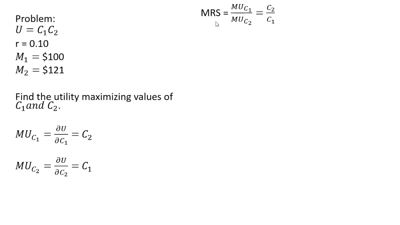
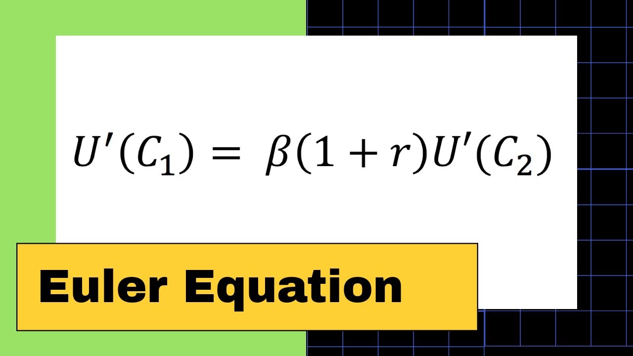
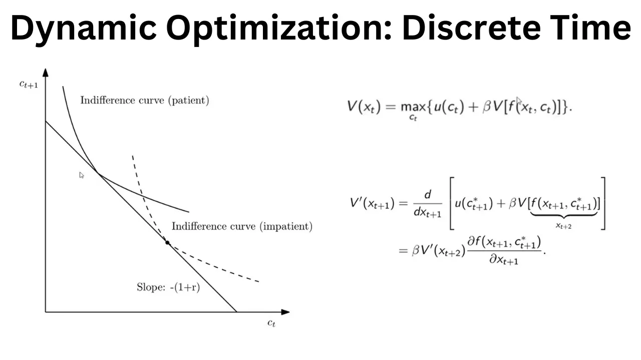


















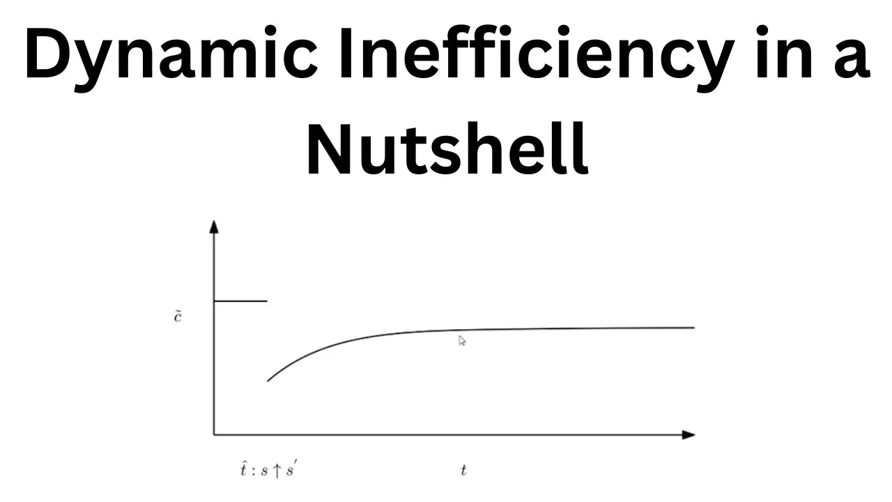

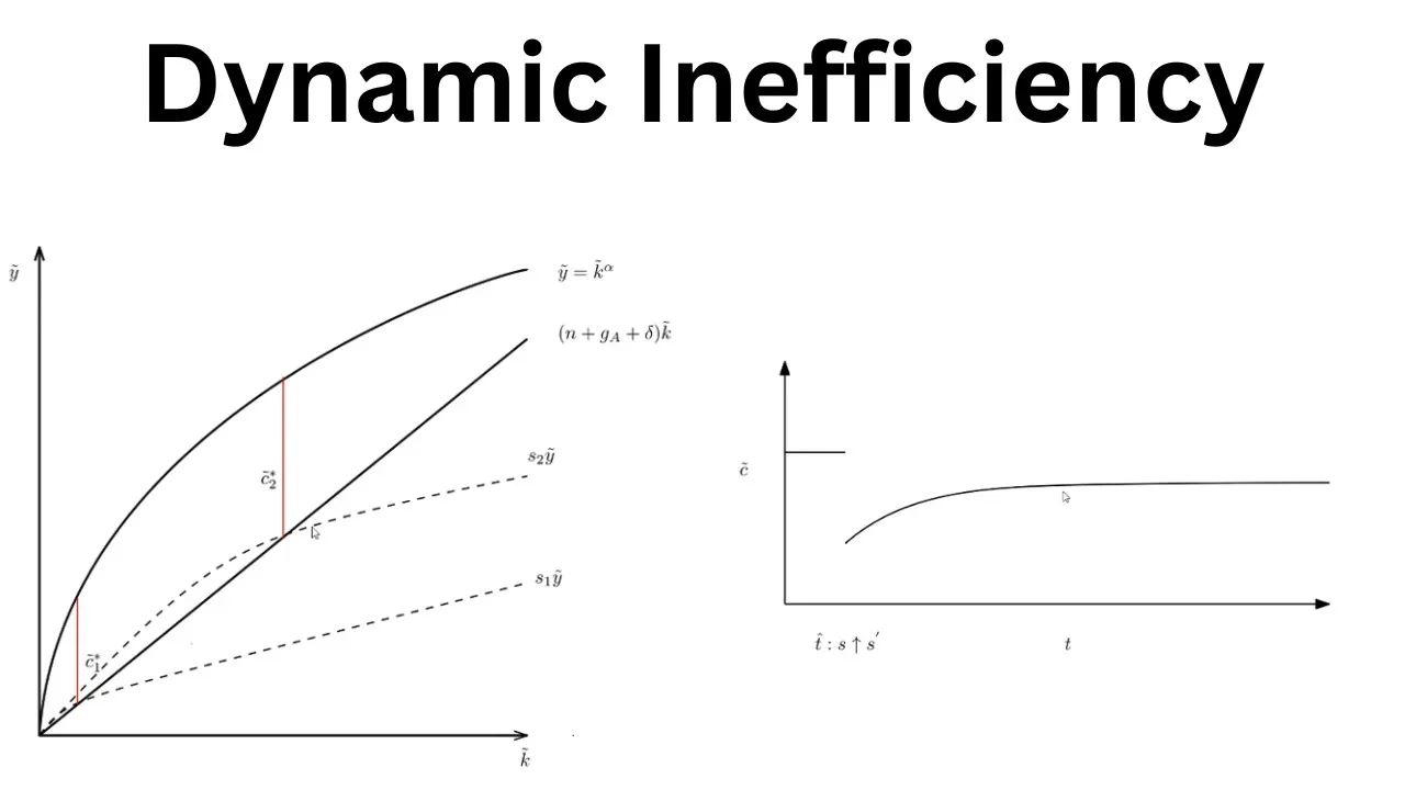

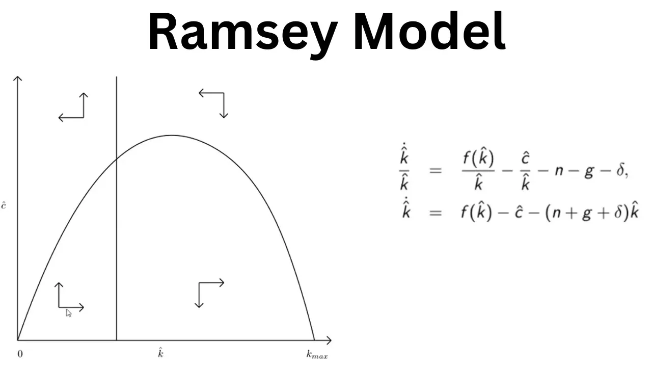

The Overlapping Generations (OLG) model, developed by Peter Diamond in the 1960s building on Paul Samuelson's 1958 work, provides microeconomic foundations for understanding long-run economic growth by modeling heterogeneous agents—specifically young and old generations coexisting and trading with each other. In this model, young individuals work, earn wages, and save for retirement while old individuals dissave, creating a dynamic capital formation process. The model demonstrates that decentralized markets may not achieve the socially optimal outcome (the Golden Rule), as the social planner who considers intergenerational welfare may choose different savings and investment paths than individual agents acting independently. This framework is particularly useful for analyzing pension systems, asset pricing, and policy interventions that affect generational equity and long-term economic welfare.
Overlapping Generations Model: Full Lecture on Macro Basics
Added:sometimes there is no intuition that's the problem of economics we need to be able to explain what we do and this is why this is such a wonderful center ok good morning welcome to the third lecture of introduction to macro advanced macro analysis and today we're going to talk about the overlapping generations model in full-blown detail so you will remember we started the course with a treatment of the basics of the supply side of the economy in the long run we've talked about capital labor and technical progress and how they interact to produce economic growth and in the long run the olg model is an attempt to bring micro economic foundations to this process the idea is to understand how conscious decisions by households and firms can lead to the processes that were formulated in the solo model in a fairly mechanical and ad-hoc way today we're going to review the last lecture briefly and then I'd like to go into the overlapping generations model in detail describing the building blocks which should alert you to the general purpose of model is organize our thoughts and we want to organize our thoughts in a way that map into what people agents economic agents households and firms do and they have preferences they used different forms of technological relationships to produce goods and services and bring those to the people who want them and that's what the markets for so we want to understand that in a very basic level and see how that interacts so we need to discuss those things in detail then we'll move on to describe a market equilibrium in which generations interact with each other and that's the whole point of calling an overlapping generation model is to show that in a very fundamental way there is heterogeneity in this model so this is not a representative agent model at any point in time there too generations alive that have economic interests in trading with each other and there's an old generation and a young generation and that's also quite interesting to to apply it's useful to apply to our current situation because these the relative weights of those two generation those two generations the old and the young at any point in time can change and that would be fundamental to understanding the the appeal of this model as I told you last time this the model we're discussing today was developed by Peter diamond in the 1960s but in fact it's it's an extension of Paul Samuelson's epoch contribution in 1958 the overlapping generations model of money - later on in this course will use the same model - to show how money worthless paper or any sort of worthless trinket that people agree to use can be exactly the mechanism that moves an economy away from an autarkic equilibrium - one in which people trade with each other in this model capital is being traded so the the fundamental means of payment is actually an asset which is productive and its own right so we won't see this so clearly but it's useful to start to think about this generational structure initially and then we'll go back and rediscover all this is a prescription by a central planner who had an objective in mind in the in the solo model it was maximizing consumption per capita in the steady-state and again the insight there is that per-capita GDP is not an objective per se what matters is really what people consume out of that GDP it's we've got a big GDP which were just reinvesting at a very high rate it doesn't really benefit anyone it benefits some empty notion of producing lots of goods and services but not necessarily goods and services that make us happy in the end so that's why the golden rule is such an interesting concept we used the Samuelson with a solo model as an approach to to doing this the Samuelson inside or the the Samuelson diamond inside would be to use this model to think about the market's ability to reach this Golden Rule on its own and we already saw the Solow model need not reach the Golden Rule on its own and I'd like to give you a very important intuition as well the the approach of this of the golden rule is to ask the question what would a social planner do if a person had the ability to actually do as well as or better than the market by some sort of planning rule or planning decision what would that person choose what would you do and that is not necessarily advocacy for central planning but it's just a question that economists are free to free to and quite to ask and to answer to the best of their ability under the constraint that they the problem is actually one that can be solved so a lot of people have criticized a social planner concept because it it doesn't seem to have an analogue in the real world but we do we can't imagine a world especially today with digital technologies that these types of planning central planning decisions would work considerably better than they did in the 1920s under the the Soviet Union and even if we don't think it's a great idea we can still ask the question can the market actually come close to achieving the theoretical first best and then we'll use that the insights we get from the oil G model including its imperfections because the OLG model will not necessarily reach the first best it will necessarily replicate the social planners optimum we can ask whether policy can improve the outcome and we'll have two nice examples to conclude with okay so let's go to last week's analysis we we finished up the solo model we discussed the the notion of comparative statics it's a very important economic concept in both economic growth and other types of economic models the idea would be what is the consequence of changing a particular parameter that is given to the agents and not really movable we ask that question because we'd like to see if changing a certain fundamental assumption might actually change the outcome and that the comparative statics analysis has proved useful over the past 150 years of economic analysis and we'll do that we did that with the solo model and showed that you can change parameters like the rate of depreciation the rate of technological progress the savings rate of economic agents the grade of population growth and trace through the effects on economies if you like across it a cross section so we could use this model to explain why some countries are rich and some people some countries are poor and we also noticed that the model has implications for how long it takes to reach the purported steady-state that we're looking for and it turns out that's a very slow rate okay and keep that in mind when we talk later about other aspects of growth models we also talked about the golden rule and we talked about the golden rule in the context of how much you have to save to reach this optimum even though that is not optimally chosen to move towards a model we're purposeful agents choose savings behavior we need to actually ask how the interest rate incentivizes agents to save or not and then we have to ask how the interest rate comes about in a freely functioning neoclassical model where the savers and borrowers demanders of capital interact in a market with with frida price determination so this would give us the gave us the motivation of looking at the factor price frontier sort of invented by Paul Samuelson a long time ago as a way of thinking about neoclassical functional neoclassical income distribution meaning if actors are paid their marginal products what kind of factor price outcomes could we observe and it's very intuitive we assume a production function that has constant returns to scale the Oilers owners equation for functions of linear homogeneity implies that basically factors paid their marginal products will effectively exhaust the output of the economy so that very fundamental equation will guide us through most of this course because we will be assuming that the economy is fundamentally characterized by constant returns to scale so if captain labor received their marginal products in a competitive setting then there will be no excess profits profit of capital be it high or low is exactly equal to its marginal product in production this is a benchmark we should keep in mind and I urge all of you to study the derivation of the factor price frontier because it is really the the heart of neoclassical income distribution theory and even if you don't like that even you'd like to adopt a Marcia and Eris wrothian or some other notion of income distribution or monopsonist view you still need to understand what you're criticizing so this is the benchmark against which we compare perhaps more realistic notions of income distribution and then we would into the introduction to the the diamond models this lengthy introduction today is to to get people revved up for this fairly technical model at least for many of you economics is still an ocean of graphs and not necessarily of formal methods this is to get you thinking about microeconomic foundations so we will discuss explicitly preferences will discuss technology market form equilibrium and then compare equilibria across different parameter constellations okay so let's let's continue that discussion now remember the OLG model is designed to implicate to study the implications of private behavior on a public outcome which is capital formation and the associated growth dynamics that we associate we put on capital formation the best example I can think of right now is China an economy with very high savings rate very high rate of economic growth compared to its own past and compared to the rest of the OI the developed world and the developing world and try to make some link with economic welfare at the same time and we can do that because we're looking at individual households the the felps problem of the golden rule the modified golden rule we're always choosing consumption per capita and even that's not necessarily a desideratum there may be a cost associated with more consumption per capita that are not really well covered in the in a model without looking at the utility of agents and the relative valuation of increments to consumption and that's we're gonna do today we're gonna actually get into that into detail so these models therefore can be used to think about policy we can also use it to think about uncertainty this model will not have labor supply that's endogenous but you could easily put it in you could easily add a be' quest motive this the quest motive could be motivated by the desire to make children and offspring in general happy as happy as possible it could also be used to extract behavior from children all these things have been done before we're gonna you know you even think about unintentional bequests because no one really knows when they leave this this this earthly existence so all these things can be incorporated so the model is really a baseline I'm trying to make a basic point to master students and for those who are interested this would be a great place to start picking up the pencil and paper and trying to do this on your own this model has great implications for pension systems it's been used in a more detailed from a form to look at those questions moving from pay-as-you-go system to a funded system or some sort of mix thinking hard about why you'd like to have a mix instead of having all capital based or fully funded pension systems or fully owe as you go you can use this model to think about labour taxation and its effects you can also think about asset pricing and the implication of asset price bubbles possibly unsustainable evolution of certain prices and the effect that it has on the real economy and such such models and also think about as I said before altruism so let's go quickly into the notation remind ourselves what we're dealing with they're dealing with an economy that is growing and I'm gonna shut down technical progress for the time being so we'll deal with a static production function but growth is still happening and turn in terms of GDP because we have growth of the population so think back of the Solow model the economy's fundamental production factor is population which is employed and for simplicity we'll just put those equal to each other this is a full of full employment economy and we'll consider the rate of growth of that massive input and as little n so the land is the growth rate we're dealing with a discrete time model so you can think of the population in a point in time solving a difference equation the current value of LT is equal to sum L 0 times 1 plus n raised to the T power ok so that's this would be the solution to the difference equation all you need to know is T and then you know what LT is ok so that's gonna be the source of growth in our economy and as a result successive generations will be larger in size and they will continue to exert pressure on the on the environment if you will this is a great model by the way for looking at environmental damage it's been done before but there's all lots of new interesting work to do if you think that there's a finite resource think of the environment think of the the global temperature the carbon burden of the economy as being a finite resource than every future generation in increasing numbers puts in excess and an increasing burden on that on that fixed resource there may be some sort of tech progress that offsets it yeah that's what you put in the model is what you're gonna eventually be able to to tickle out so no further comment there but the key thing is this the next line which deals with the the generational structure any point in time T there are young and old people around and both of them have interests in consumption see one T would be the consumption of those who are currently young and see two T would be the consumption of each person so per capita of each old person in period t okay so these these are simultaneous claims on resources that are being produced now obviously C 1 T and C 2 T are different people people's consumption so their planned by different people and they have different interests and the old person's consumption C 2 T is will correspond to someone's decision in C in in t minus 1 so the C 1 t minus 1 is basically the the consumption one would associate with the person who is currently old consuming C 2 T now in when you're young you sit you do some savings you don't say when you're old because there's no pension there's no request lot motives so people won't do that they'll just basically dis save so within the economy at any point in time you have just saving going on and s T is the is the savings by the by the individuals in period t by the who are young okay so that's one of their control variables if you like to decide as they move forward with a view of creating enough resources for that particular individual in period 2 of their life when they become older and T plus 1 we're going to assume that wages are paid to those who work and labor supply is inelastic so they'll be exactly for each individual household Omega t available from which savings can occur or consumption can be paid this is a money that's economy so we're talking in any period of time we have a single good the only differentiation of goods is the good is a differ a ssin of goods over time as they are carried forward as potential productive production productive assets capital so Goods can be converted into either consumption or capital and back and forth and then this these Goods once they've been sort of nailed down using production they get used up at a capital depreciation rate Delta so we can think about already if there's a market out there you can think of the market paying a gross rate of return on savings that are decided in period t and this you think about this as I mean one way I like to think about this is you you save by buying a Mercedes Benz and then you you sort of rent it out to some taxi company who drives it around the city for a while and gives it back to you in the second period and then you can trade that in for some consumption and that car you getting back will have depreciated a little bit after it's been used in in in service as a capital good and that would be thought of as delta x kt so what actually remains for the person as a mass of resources for consumption the second period has to reflect that so it'll be 1 minus delta plus whatever productivity that at the margin was generated by that capital good and that's going to be given later we'll see but as the marginal productivity of capital in that period okay so if you think about it we can easily concoct a net interest rate by subtracting 1 from that capital r it's just kind of like the what you get on top you get the you get something like the car back maybe run down a little bit you're gonna literally want to have a bit of compensation for that depreciation ex ante maybe you won't get it the market clearing price but in the end Ortiz is gonna reflect to you compensation also for this loss of capital that occurs through use in production okay and then you have your inpatients so we're gonna write down utility in a second it's gonna reflect utility over two periods consumption when you're young when you're old and you decide when you're young and beta is gonna be the relative weight you put on future utility so it's one divided by one plus some sort of some sort of private rate of preference some sort of subjective discount rate if you like okay so it's a you know if beta is very close to one that would mean that we're pretty pretty patient we're willing to to to wait for consumption in the future and if beta is low that means we're impatient we have a high implicit social or sorry private discount rate or rate over time preference okay so to get to get moving we really have to move talk about the the way these factor prices are determined in the decentralized economy so we need to consider firms which use the factors of production economy they're two of them capital labor and there are price takers price meaning factor price the price of labor is the wage the price of capital is the the rental rate we talk about the gross rental rate because the firm has to basically return the capital good at the end of the day to the to the owner and constant returns would imply that they with the maximize profits they pay factors their marginal product and there's no excess profit for any firm regardless of the scale so we can talk about a representative firm the scalability of firms in this economy is is completely it's completely flexible there's no decreasing return at any margin so we can speak of a representative firm it doesn't really matter to us okay so having done that we can think of all the potential combinations that a firm could A two factors these two factors under these assumptions okay so think of the profit maximization problem and in section you will have seen this and I urge you all to do it on your own because it's a nice derivation to think about what a profit-maximizing firm can it effectively afford to pay its factors so one way of thinking about it's just a maximization problem given a wage what can the firm afford to pay the other factor who gets a simple type of problem you can think about think of the what is the maximum wage a firm could pay given a rental rate it pays on on capital so the to two different perspectives are the same problem okay and the answer would be this curve this curve which is con convex to the origin and that means that any ray that connects two points on the curve those points along the Ray are lying above the curve okay and the origin is in the corner so you can see immediately that the higher the wage that a firm can would pay to to to its workers would necessarily imply a lower rate of return or rate of of rental net rate of rent rental rate on capital and that just falls out of the availability of resources of a profit-maximizing firm to do to pay that to pay that rental so you can imagine various points along the curve and then it's easy to show with calculus that the slope of the curve at any point is going to be exactly given by the capital labour ratio and production okay so it's a nice demonstration that you will see in the section okay and there's it's it's actually a very very simple elegant proof and you can see right away that if we choose a point on that curve which is determined by technology by the way if we choose a point on that curve that has a very high wage the low capital rental rate will necessarily imply a capital labour ratio which is high if you choose to the contrary a point in the lower southeast you'll have a a low wage a very high rate of return on capital kind of makes sense but implicit will also be a very low capital labour ratio okay so labour will basically be used much more intensely intensively relative to capital given those factor prices okay that's a name you know one way of thinking about what happened in Germany for example Germany's be known as very very capital intensive company country when I was when I first came here in and before and in the in the course of the hearts reforms the the wage level at the median and at various quantiles of the wage distribution has fallen in real terms and you can really see looking at the German discussion there's been more employment less investment it you can think of this whole process is just reflecting movement along a factor price frontier at the same time one one met one cannot forget that this thing will move over time and we have technical progress more and more output is possible with given wage the this given capital and labor combinations meaning that as we move through time holding one of those factor prices constant would make it possible to pay the other factor more and more so keeping the wage constant means the profits start to rise keeping the the rental rate constant would imply that wages could also rise or you could have some combination of the few of the two okay so if you add depreciation to this you're doing nothing more than just slicing off or hiding off a certain amount of output for the replacement of capital so we could think of a net output relationship and the wage and the rental rate reflect positive depreciation previously I derived this curve mentally using with without appealing to a crude depreciation at all okay so it should be clear to you that a high depreciation economy there's going to be less output in net around to make us to make us happy with consumption or to to provide us with investment for the future okay so how do how do agents how do house who by the way own the capital okay so even though the households know that they can't really influence the general equilibrium we're just gonna behave as if they're priced acres at every moment they are responsible both for supplying the labor and supplying the capital and we don't make any statement about the distribution there's no wealthy class in this model that owned all the capital and the workers do all the work this is a representative agent model so keep that in mind very important benchmarking economics one that has become somewhat critical and criticized in developing future insights on how the economy actually works we think that economies with distributional issues may actually behave differently think about optimal behavior in this economy think about a savings decision of the young generation earning Omega wage for an inelastic supply of labour this household is gonna supply one unit of labour come hell or high water because that's all it does in a more advanced model you could have some endogenous labor supply households might want to work harder if the wage is high and work less if the wage is low but let's start with the basics so we're optimizing the outcome for the household we're choosing the best possible outcome for a household as a solution to this problem this problem basically states that utility is the is a separable function of E - of consumption today in consumption tomorrow and I'm choosing my consumption today and my consumption tomorrow as a young person in this economy c1 t is current consumption c2 t plus 1 is consumption tomorrow I can't do this without constraints and in a market version of this model I have to obey the following constraint what I consume tomorrow is exactly what I earned today less will I consume today and then basically multiplied by the the rate of factor payment and we'll get on this savings as a capital good in this period okay and we're gonna assume that these utility this utility function is time separable I already said that and this common Felicity function or time sort of temporal utility function at any point in time is the same it doesn't change over time its first derivative is positive second derivative is negative it's a concave function of consumption now we can basically use the lagrange approach to the sub to solve this problem we can also just just do brute force and and and use the constraint to eliminate one of the choice variables so i will rewrite the problem is simply a choice of savings today right by choosing my savings today given that i'm working one unit of time earning omega means i've already decided how much i'm going to consume today because what I don't save I can consume and I'm not going to throw resources out the window and what whatever's basically saved will accumulate will yield to me in this perfect foresight model okay I know what are our t plus one is even though it's going to happen in the next period that's the the benchmark perfect foresight version of the OLG model means that I know exactly what I'm going to be able to consume tomorrow which is our t plus 1 times st okay so it's a very simple problem that anyone who knows how to do calculus can solve okay and the utility functions make it very make us confident that we don't have we're not gonna have multiple inflection points we're not going to have different we're not have any further choice as a Maximizer we just choose the inflection point and make sure it corresponds to a maximum utility so we'll look at the second derivative with respect to s make sure that it's that it's negative and basically we've solved the problem there's no bequests mob motives in this model so it's a very simple problem to solve and everyone should be able to do it I knew andreas does this with the Log form of you you should be able to do with other forms as well linear quadratic or things like that the first-order condition is a single first-order condition it says the marginal of consumption today is equal to the value of utility I get from that savings that we'll consider as an alternative evaluated at the marginal utility of giving me margin utility tomorrow evaluated at the consumption tomorrow and I'm going to discount that back using beta okay so if I if I save one unit of consumption I lose some utility today I get it back tomorrow and I get RT plus one units of that and I multiplied by the marginal utility of consumption tomorrow and I discount it back using beta it's a very simple problem we'll see this in macroeconomics constantly it's basically a version of some sort of optimality conditions we call it an euler equation in a multi period model or a Euler equation as some Americans say French would probably say oh well all right now equation anyway sometimes you have to laugh at your own jokes at the optimum it's it's very intuitive okay so it's kind of a variational argument by move consumption around the margin I'm not gonna make myself any better I'm at the top of the hill so to speak when we're thinking about this problem is this like a mountain and when you get to the mountain you can look right and left back and forth and you don't see any gain to moving away from where you are so you've reached the top of the mountain its way of understanding this problem okay so once having done that we can either solve directly for a consumption and savings function given the wage today and prevailing return to capital expected to prevail tomorrow and we could look at changes in things the agent takes as exogenous including the the factor prices okay so we can we can use calculus to tease out the reaction of optimal behavior especially savings that's the most important thing how does a household respond to changes in the savings rate we can write a consumption function if we're lucky we can write it in closed form so we can write consumption as a function of stuff on the right hand side or we have to look at the local behavior of consumption as a function of the current wage you know with the mind of the fact that it may change as we move farther away from what we started so we're going to write a savings function as the outcome of that exercise we're going to use the capital when you use capital S as an indicator of this function it's going to be a function of two variables it's going to be a function of the wage and it's going to be a function of the rate of return on capital in the following period and this is going to characterize the behavior of the currently young generation okay and it's easy to show it's easy to easy to show that the first partial derivative with respect to the wage is positive for all values higher wages will lead to more savings because you want to consume more tomorrow as well as today so you'll spread your income across the two periods the curious part of this problem is is the ambiguity of the second of the second argument the first partial derivative of s with respect to R can be positive or negative depending on whether the substitution effect or the income effect is larger generally we'll assume that the substitution effect predominant will dominate the substitution effect means that an increase in interest rates makes consumption tomorrow cheaper so we want to save more today but at the same time an increase in interest rates might make us feel so rich that we actually want to save some more today save less today because we consume more today so those two effects may actually cancel out in a in the case that andreas talked about the log utility function case the periodic utility function being log would imply the day X would you cancel out so increasing interest rates for the in the log case has has neither a positive nor negative effect on savings today but in general we think empirically that there's a slight positive effect you ready this can also be shown it depends on the initial allocation so you know a very wealthy household will probably place more of more importance on our increase in interest rates in terms of its accretion to its ability to consume whereas a highly indebted household will have a very negative view of an increase in interest rates so think about that take the simple case alluded to already log utility do it as an exercise you will have done it in the in the section already the next step is to look at equilibrium so we have a supply and a demand and it's easy to see that what's demanded by the young as savings as gross savings must be somehow supplied by the old people who put aside capital put aside income as capital and didn't consume it owned it and they are trying to cash in it doesn't make sense not to cash in when you're old because you're not gonna get anything from having a owning a factory when you're dead so you will use that to increase your consumption when old okay so this equilibrium condition is extremely important it's also giving us an equation of motion if you like for the capital stock over time okay so you can see the capital stock tomorrow will have a relationship with the size of the population it seems to be pretty clear big big populations Keter asparagus will want to spend more but they'll also want to save more so it'll be more capital tomorrow all things given and it will also depend on this savings function which is the per-capita behavior of young young people okay so we divide by NT plus 1 we can rearrange this nice equation to look like a per capita per capita equation so it just says that it's equal to the the behavior of the individual household when young normalized by the fact that in the next period will be more of these people around so to if you want to understand how the net per capita capital stock is evolving you have to account for the fact that next period there there will be more of these young people around and that will sort of dilute the per capita value going forward okay so at the moment we're going to assume perfect foresight as before and therefore we can think of this growth capital return as simply being a deterministic function of the of the savings behavior in period t and the population evolution so we can we can think about it when the firm is is doing the best it can given its technology it's going to pay it's going to be willing to pay given its capital stock that it has to work with it's gonna be able to pay its marginal the marginal product of that capital stock and that market that capitalists was supplied in elastically in period 2 into period t plus 1 so that our t plus 1 has to be equal to 1 plus the marginal product of capital t plus 1 less depreciation on that capital going forward and we can just rewrite that by substituting but we've just derived as the capital stock per capita and T plus 1 and then we have this this nice equation for the the rate of interest the net rate of return on capital the net user cost of capital going forward okay so we have two relationships that are actually independent of each other between our the rental in capital and the wage Omega okay there's an inter temporal break between the two but in the OLG model we're gonna spend most of our time in the steady-state so we'll want to know where we're going in the long-run as the economy converges to something sensible and we're gonna have to ask whether this equilibrium actually exists so to do that we need to look at the slope of this relationship to make sure that it's slope the right way you'll see what I'm saying in a second but the the classic way to do this is to take a curve and take a total differential of that curve with respect to its two endogenous variable see what what shapes that that slope okay we're gonna compare that slope to the slope of the the factor price frontier because that's the other relationship this this relationship that the market equilibrium the goods market equilibrium curve people that people like to call a blonde shardcall to that with Fisher and they're in their epic textbook I'm gonna stick to that oh just called a goods market equilibrium because there are two markets in this economy and this one this is the one we're gonna focus on okay so this curve is has negative slope and it's negative for sure if people respond to an increase in the wage the way they're supposed to do they save a little bit spend a little bit and then if savings responds the correct way if the substitution effect dominates okay this is only a sufficient condition it's not necessary but if you have to really cook it to make everything work out otherwise so we're just going to assume that these conditions are met and if you want we can meet in a bar somewhere and discuss these other conditions okay because there is this issue as we've seen in the German discussion that maybe an entry increase in interest rates may actually lead some people to consume more because they have lots of savings but for this economy with a representative agent I think it's pretty pretty okay to to do what the literature is done which is to assume the the substitution effect either dominates or is offset so you know SR F sub R is equal to zero the the model still has a pretty acceptable characteristics so let's plot these two equations very quickly to describe the goods market equilibrium this is a course where we spend a lot of time with graphs just to reinforce intuition and the intuition can be extended or even expanded using mathematics okay so this is you know wages and capital return moving in inverse directions for a given technology for two different reasons okay and this is the the goods market equilibrium reason and the other one we've already done which is a factor price frontier so we're done just have to intersect those two curves okay so make sure you understand where this one comes from I put the equation here just to remind you and then we've got the factor price frontier and then we can discuss steady states must be the intersection of those two curves when our t plus 1 equals RT equals R star and Omega T plus 1 equals Omega T equals Omega star and if that's the case then the capital labor ratio has to be constant and that's going to be called capital little K star okay so just like in solo we have an interesting setup if we did have technical progress we actually have some per capita income growth we've shut that down on purpose so just in your mind put a equals 0 but this is the same condition that we had with solo the capital labor ratio is constant but capital is growing at least a traitor and okay and the wage per worker is growing at rate a which we have set to zero okay so if you like just just think of a equals zero going forward but this model is extendable so we can do more with it if we want but we're gonna keep it keep keep the ball play the ball low to get this get this through okay so the intersection of those two curves gives us the green dot the green dot gives us Omega star and our star so we're done and you can see probably why the slopes of those curves are important we want the goods market clearing curve to be steeper because otherwise if we have a temporal dimension to the adjustment to equilibrium we won't have a convergence to the dot we will have an explosion away from the dot okay and to see that you can you can think of the model is actually characterizing a difference equation a linear or a non linear first order difference equation in this particular case and the case we're considering it's going to be nonlinear and we can linearize it to characterize it's it's local behavior around Luque star all we need to do is just plug in the equilibrium values given by the factor price frontier and those need not correspond to the steady-state but if there is a steady state we will eventually reach it so you can see that KT plus 1 is a function of little KT through the factor price frontier and also it's a function implicitly of KT plus 1 because that determines the marginal product and of capital in the in T plus 1 as well as the rental price of capital in t plus 1 ok so we have this we have this nice implicit relationship between KT plus one little KT plus 1 and little Katie ok but of course it's not linear so we stick with a diagrammatic exposition for a few more minutes and then I'll do quickly the linearization trick very important in macroeconomics most of what we have in macro is not linear so we need to we need to take seriously the behavior of the model around as an approximation approximated model around the steady-state okay so to to sort of think about stability we just need to ask what would happen if we were at that green dot characterized by r1 Omega 1 and the red curve would imply that basically that can't be an equilibrium but it would wouldn't correspond to a point on the factor price frontier so it wouldn't be consistent with firm behavior that to make it consistent with firm behavior would have to would have to observe Omega 2 but Omega 2 would imply less savings and that would imply a higher interest rate so we'd have to move across from Omega 2 to R 2 but that's also not consistent with factor price equalisation Tirek behavior by the flirt by firms so that would bring us down to the to the blue curve again and basically the logic of that would be to show that we have to be a w infinite w infinite doesn't mean infinite time it just means basically at any point in time if you if you iterate the logic of those two curves they cannot be consistent with each other unless we've done that iteration and in phenomena of times and we've actually reached that green dot so that green dot is supposed to characterize at any point in time to be hit the steady state behavior of the economy okay for a given set of behavioral characteristics okay similarly you cannot make the argument that if we had a lower wage than the steady state dot you'd expect basically a rate of return on capital it's very high and that would induce more savings which would induce higher wages which induce more capital formation which would take some of the edge off the higher marginal product it would still be 2i so we still have more savings wages would continue to rise until we reach the dot characterized by Omega infinite and little R in fit okay so these are just these are intuitive arguments to show why a stability condition like this the absolute slope of the red curve the goods market equilibrium has to be greater than that of the blue curve the factor price frontier okay and you can you can basically look at the the calculus around this you can take a total derivative of that dynamic nonlinear relationship and solve for the local behavior of KT plus one gate given KT okay that's one way of doing it and stability intuitively would say that if I perturb KT a little bit we don't want KT plus one to be bigger than the perturbation went to be smaller so it'll sort of iterate back to where we started and that's exactly the intuition that this equation gives and we can show that formally it's but it's exactly the expression of the relative slopes of those two curves okay so if we want we can do this formally the two ways of doing I'll go very quickly through them very essential for my economics okay so one is to to differentiate that relationship totally I just said that so the the formal step would involve involve basically holding everything else constant and just taking a total differential of that the first expression and getting KT DK t plus one small changes in KT plus one as a relation in relation to changes in DK T and of course you see the the implicit relationship because DK T plus one is on both sides so we need to solve and we get this beautiful relationship as before okay that's the one way of doing it and the stability condition you can find it in many textbooks it's basically a the assurance that the model does not explode in response to a small perturbation of of the economy from its equilibrium be damped back to its stationary state this is not guaranteed I can cook models where this doesn't hold and it's not clear they're very interesting so the standard benchmark case we do in the section with cobb-douglas utility sorry log you logarithmic utility and a cobb-douglas production function will guarantee that the stability kate condition is met but there are many many other model specifications that also satisfy the stability condition we can do a similar exercise which comes into play later on in this course we start doing dynamic macroeconomics to start doing dynamic stochastic general equilibrium models of all different flavors and then this is called basically log linearization so it's the same kind of idea instead of taking a total differential you would look at the behavior of the model in terms of percentage changes around its steady state okay so you have to identify the steady state and ask for the response of KT plus 1 as a percentage change in response to a 1 percentage change for us unit percentage change of kt okay so the nice thing about that approach is that we have something already that has no units we think of Anna last elasticity environment which is useful for economists who want to compare the behavior of Germany Sweden in the United States these are very different sized countries but we have this feeling that maybe economic laws are kind of size invariant and a lot of what we have found is actually confirmation of that so this this economy should be this this model of the economy should be equally valid whether we look at a small open economy or a large closed economy under certain conditions that's the that's the intuition that one would get from using the log linearization because small changes of logarithms are like percentage changes of the original variables okay so let's do that very quickly and this is really meant to be a signal to you as to what's important for your future if you choose to do macroeconomics as a field you need to be comfortable with this type of approximation first order Taylor approximation of logarithms of relationships so we take natural logarithms of both of those of the both sides of that equation we're going to get something that looks like this so that's not very hard to understand we need to identify a steady state and look at the changes of that object with respect to the steady state which doesn't change by construction okay so in the steady state we have we have that equation holding ok so that's a static that's that's like a rock doesn't change at all so we're gonna ask really how does the how do small perturbations of the first compare to this okay so if we subtract this this equation 3 from perturbations in equation 2 we're gonna have literally changes in the logs of all of the variables that excite us and those can be thought of as last percentage change responses to percentage change responses it turns out we'll get the same equal the same stability condition it's just a different way of looking at it okay so we keep in mind that these two relationships characterize the the curves one is the factor price frontier the second one the first one is the is the goods market equilibrium condition at any point in time t plus 1 then we're in business we just have to do the first order Taylor approximation so it sounds awful but every master in economics knows how to do this in the shower if you don't you don't earn the name master so go back and remind yourself what a first-order Taylor approximation looks like and it looks like that okay okay so we're talking about approximating the left hand side and the right hand side and then subtracting in equation 3 in Log form from both sides and rearranging see what you get you get something it looks like the percentage change it's approximately equal to the log of KT plus 1 divided by K star okay but this is a really convenient way of thinking about it's like the little percentage deviation dividing by a hundred to get rid of the percent as a function of the percentage deviation or the fractional deviation of KT from K star in the in period t okay so and that constant of dependence is exactly what we had before okay so keep that in mind it's a linear difference equation and it's not a differential equation we want this this this relationship to be less than 1 in absolute value and how do I know that this thing has the right sign well f double prime is the second derivative of the production function that's supposed to be negative by assumption we have decreasing marginal product of capital so the minus times the minus gives us a plus okay and I got this object which will be positive if the savings rate responds the savings function has the right derivative the sign of the derivative with respect to two R is positive and the minus and the negative second derivative of the production function cancel out okay so again the same condition we had before as I said before we've already assumed that consumption in both periods are normal so increases in income will correspond or result in increases in savings so that consumption can increase in both periods and we just will just assume that savings is a positive function or a non-negative function as a sufficient condition to get this thing to work to work okay so now we've got policy examples we we can do this very quickly the great exam question say that again what is the effect of changing a parent parameter in this model trace through the changes which curves shift so we could think about a change in patience and increase in patience would be a drop in the discount rate the subjective discount rate or an increase in the discount factor you put more weight on utility tomorrow so you'd want to do more for your consumption tomorrow because it's more valuable to you you can also think about changes in the depreciation rate changes in the growth rate of population changes in the rate of technical progress were we to have it in the model remember I've just set it to zero from the beginning for simplicity okay so we'll take an example and this gives you the advantage of using a curve approach graphical approach to solving these questions as a first cut and then you can ask the hard questions is this robust you can't always do this in economics and later on in advanced macroeconomics you can't do it at all you're gonna have to use the computer and it's a bit frustrating because sometimes you want to have intuition and intuition is often served [Music] you sometimes there is no intuition that's the problem of economics we need to be able to explain what we do and this is why this is such a wonderful setup so this is a great a great intuition generator for understanding why and increase in depreciation which what one might naturally associate with the with the internet economy the which considers software to be a type of investment but it doesn't last very long it's not the same thing as building this building a situation like that would would correspond to an increase in the depreciation rate in the economy now of course this is a an abstract mental experiment obviously the the economy in Germany is dominated by buildings as it is in the United States so an increase in depreciation rate resulting from the internet revolution might only be marginal at the beginning but over time as people invest more and more in this type of technology the role of this depreciation rate might change on the other hand in the long run we still need to live in houses we might live in worse houses but we're gonna live in houses with my live in better houses but given the technology we have today an increase in depreciation is not such a great thing okay it means there's less national product for everyone to share so the factor price frontier is going to shift inward so at any given rental rate on capital that we could generate there's going to be lower wages or any given wage we're going to be able only able to pay capital less and to understand the general equilibrium we have to understand what happens with the other curve we can't just assume it it's constant we have to look carefully at it and that's a little bit tricky it could actually shift outwards and if I'm honest economist you have to consider that case but if you look carefully at the using sort of comparative statics arguments the more likely shift will be inward and you can discuss that in the section if you want they're sort of off off-the-wall conditions would give you an outward shift but if it's an inward shift the answer is unambiguous that both factor prices will decline for small changes and we can be relatively this is kind of a good characterization we have today you can think of this as part of the part of the the whole the plate or the platter of problems that we face with with with secular stagnation there's several things going on one is population growth is declining the other is technical progress is slowing down so little a should we consider it as slowing down so those would also kind of make you expect that the rate of return on capital would drop real interest rates would drop but it also means the wage will slow down or drop okay so this is kind of exactly what we've observed throughout the OECD in in the past 15 to 20 years so this could be a pretty legitimate explanation of what's going on now is this the best we can do I alerted you to the beginning that economists that are honest have to ask the the the optimum question is this the best we can do is the market really going to give us all the things we want and there's nothing wrong or immoral with asking that question because personally I think the market does a great job of allocating resources competition is great we need to make sure that we have competition we need to make sure that markets are transparent but we still have to ask the question can we do better okay and the reason we might not do better is because the individuals that are discounting may not have the same rate of patience that the social planner of the government or some sort of moral instance the moral judgement of generations aggregated might consider it unfair to take decisions that have effects on future generations without having the future generations at the table and because they're not born yet we can't get them at the table we can only act in on their behalf this is a deep deep point which has been raised many times especially with respect to environment and Environmental Protection or global climate change to the extent that it is happening and I'm pretty convinced that it is happening the question is you know what does humanity's role and I think I'm more more convinced that humanity's role is not negligible and there are lots of nice examples of where this has actually worked think about fluoro chloro hydrocarbons in the atmosphere is a great example of our global cooperation actually could could accomplish something so if it's the extent that we think there's a problem there might be a reason for Humanity to get together and try to change it so this is a very interesting way of thinking about though alg model right is it fair to ignore unborn generations so it's not a it's not a trivial answer may may be just fine maybe the market economy gets it right so to do this we have to set up the social planners problem we have to think about it carefully and we have to delineate the plan of action the course of the parameters of control the social planner could have I'm gonna shut down technical progress here just to make things easy but if this is no by no means necessary and I'm also going to look at this optimality condition in a perspective that may be illuminating for some of you there's a the social planner will also care about within periodic intertemporal optimality as well as intertemporal optimality so the the the the social planner treats all generations equally or treats them unequally in a way that has to do with a discount factor and that will make a big difference in terms of comparing these outcomes okay so we need to think about social welfare as being an aggregation of utilities of different generations so we're going to assume that is additive this is also nothing controversial assumption so we're gonna argue you can compare individuals in a quantitative way okay so even if we can't measure it directly we can still ask the question if we can characterize some of the some of the aspects of that utility then maybe we can still improve Social Welfare compared to the private outcome the most pressing and difficult question is how to weight the generations and this is the Ramsey problem problem that has been boiled has boiled over to discussing policy action parameters with respect to climate change how much should we wait the future generations should we have a very low discount rate a very high discount factor or should we treat them as if they're just assets and some sort of financial problem so I tend to think probably more like Ramsey but other very serious economists more serious than myself including the Nobel Prize laureate these this year seems to think differently okay so we're gonna set up the problem of a central planner this hypothetical instance of planning genius that will sort of do everything right and see how that comparison this is a very important issue and again if we're not dogmatic about it if we don't think that markets you know just the only way to do things then we should probably ask these questions because maybe through a clever tax or a subsidy we can make the outcome better for everybody alright so we use an OK notation is very similar to previous the previous case we looked at the private sector market equilibrium the private equilibrium and the only notational innovation will be the use of theta which is the central planners discount rate and this would apply to been our C's C but use a geometric weighting scheme so as time goes as as as the distance to the present increases we exponentiate the gains in the future by power of T of 1 divided by 1 plus theta the social discount rate so think about it's the social discount factor would be the inverse of 1 plus theta ok now theta can also be negative if you I'll talk about this in a second so it doesn't have to be positive if it were zero then the the social planet would would wait all generations equally but of course generations are growing in size so it's not really fair to the individuals of successive generations it's just all generations are treated equally the central planner may actually care about people like you know irrespective of the time that they're born in that case the date would have to be negative okay so the social planner she will choose yeah and it's interesting she has to also deal with the currently old people so you always have these old people around right now if he get to reoptimize and decide on a new plan you still have to deal with the current old generation because they have nothing to offer so when Social Security was introduced in the United States this was a gift to those old people who were old in 1935 I mean the people who were who are already old were getting sort of a free lunch but that's just the way it works because you're gonna basically end up transferring resources and you want to make those people happy too if you set their utility close to zero you're gonna you're gonna have huge gains if you really care about everyone and I'm just putting beta in front of them that's a convention that blonde chard uses blusher and Fisher in their book and I think it's just it's pretty arbitrary just as this problem is arbitrary okay so we're gonna use for C we're gonna use 1 over 1 plus theta and we'll make the course a reference to this data at different points throughout the rest of this lecture ok so the sequence of resource constraints and it's important to stress that the the household is not involved now it's the the planner so the planner so he understands that if the planner saves more today there'll be more capital tomorrow which will enable the social planner to produce more in in in the next period and future periods and this increase in production can be allocated arbitrarily between current generally alive people old and young at any point in time so that gives a second degree of freedom for the social plan or the social planner doesn't have to worry about what this Generation X decided to save because the social planner just decides that the people are just sort of there and there's no market such a planner is just giving them the resources to make them as happy as possible and of course we'll have to see if that thing if that policy compares well or badly with what the private sector or the private decentralized equilibrium would would come up with we also need to be very careful this is a sequence of resource constraints it's not a single one it's a sequence so each one is contingent on the one previous obviously because KT is equal to the the decision was the central planner in the previous period to save or to not to save and therefore think of this as a like an accordion or if you like it a bunch of puzzle pieces that can be locked into each other and to make one long sort of intertemporal budget constraint or resource constraint for the for the planner that would involve an initial condition of capital which the central planner has to take is given okay that's k0 plus some end of game last period end of the world Apocalypse Now type of kt plus one so I'll just say that could be either zero so at the end of the world there is nothing left or there's just some K bar can't do anything with that okay so those are the that's the in a in a technical sense that's the terminal condition or the it sort of puts a constraint on on the this chain of intertemporal resource constraints the central planner has to deal with okay so these are just remarks repeating what I said before we're gonna assume that 1 plus theta inverse is equal to C so the C sub T would be the generation T's wait in the social planners discount of utility function and again to be perfectly general theta will generally be positive meaning the central planner cares a little bit less about future generations this is like individuals being a little bit selfish or bit impatient ok Ramsey objectives of that we'll see that next week we talked about Ramsey but still if you set it equal to 0 it just means the social planner cares the same way about successive generations even though with population growth that's positive there'll be more people so it doesn't mean the social planner cares about people equally it just says that she cares about person about generations equally it's a very important distinction and if this social planner is really altruistic at the personal level would mean that actually her she would have a theta that's actually less than 1 ok that's the statement here there are some issues of when you let capital T go to infinity you have a problem because social planners optimum is just may not may not be well defined because the the objective function may be infinitely large so keep that in mind we this was a this was recognized in the 1960s by the by the people who worked on this we have to be very careful about infinite horizon problems now Ramsey was very easy with this because in some sense as long as theta is positive we've got a finite sum but when you start talking about global warming or certain models of economic growth you get into you get into issues that you need to deal with ok again the current capital stock for the central planner for her it's given she can't change the current capital stock she can she can do lots of stuff but she can't she's not almighty god she can't really change everything she has to accept some things as given okay so let's write this problem down more efficiently by substituting as we did in the individual household problem in the decentralized case we'll just eliminate C 1 T and we'll write this thing in terms of two control variables so the central planner will choose sequences of old-aged consumption for the teeth generation and capital per capita in the T plus 1 period from T equals 0 to an to capital T and again if you like Lagrange multipliers you could do the whole problem with legrasse multipliers but it's a bit more more involved and you don't need to okay so it's just substitute and solve the problem again reminding you you're optimizing that with respect to two control variables too but rather with respect to two sequences of control variables it gets really important okay so the central planner always has to think because the central planner lives a long time she's gonna think about her implications of her current decision for the next period and that's going to show up immediately in the second condition the first-order condition the first first-order condition asserts her ability to look within a period and try to equate the marginal utility of consumption for the currently alive people young and old so she's gonna try to make consumption moving between individuals equally valuable to her objective and since we're valuing all people in a period with the same sort of social discount factor with respect to her initial can initially read them basically she chooses to treat people intra temporally in a sort of a just way or at least since people have the same utility function she's not going to discriminate between old and young people second first-order condition sequence of first-order condition we'll apply to an inter temporal aspect of her decision so she will make make sure given that she's satisfying the first one that the the value of capital to utility tomorrow has the same hit with the same impact that it would have in the current period where it to be just consumed now the normalization variables there show up because we have population that's growing and we have an impatient central planner to the extent that theta is nonzero and therefore that's also going to be factored in you also have depreciation to worry about because capital today is one minus Delta tomorrow okay so implicitly weighted we have both intra an intergenerational efficiency social planner she's good and she's doing the best she can to make this again this sort of this hill climbing problem such that no incremental change of her consumption choices for currently old and young or for young today and young tomorrow no change will actually put her on a higher place on a higher hill than she's at right now or increase her elevation her altitude with respect to zero that means that she's maximized utility so satisfying those first-order conditions are necessary for her to be to be reaching the top and actually making herself as better making herself as social planner as well-off as possible vicariously the people that inhabit this economy okay so this is a really unbelievably powerful set of first-order conditions because I can met I can manipulate those quickly to get a set of first-order conditions that should look familiar to you if you're paying attention it looks like basically she replicates the private sector competitive outcome okay in one respect okay and that's the the second equation says the margin utility of consumption of the currently young is e to the marginal utility of the current of the the same young people when they become old were they to invest their capital at the rate of factory return that corresponds exactly to one minus Delta plus the marginal product of capital tomorrow that's exactly the equilibrium condition in the decentralized economy okay so if our t plus 1 is equal to that term 1 minus Delta plus F prime of KT plus 1 then we have exactly the social planner doing what the competitive economy would have done on its own so if you were if you're a market fan this is this is one point for you guys ok but I have to disappoint you it's not necessarily the whole monty you have won the game yet you've won one of the innings but it means that the certainly the the the private sector decision will give us the right relative intertemporal trade-off at the private level or the private level gives the right trade-off at the social planner would choose but there is nothing in that first-order condition that controls or determines or replicates the social planners choice of the aggregate capital per capita okay that's the that's the the the hitch if you like and it's exactly the same problem that we have with respect to efficiency dynamic inefficiency or efficiency we saw in the solo model basically there's no reason that individuals will necessarily hit the mark on the aggregate capital stock per capita okay even though they're dependent even though they're all identical there's no reason and it's easy to show that the aggregate capital stock per capita and therefore the aggregate rate of return on capital need to correspond to the social planners choice so this is exactly the golden rule and that's why I wrote golden rule reloaded okay and this was this was identified back in the 1960s among others by Paul Samuelson the so-called turnpike theorem which shows what the social planner would choose and kind of compare that with what the OLG model the diamond model with Capital samisen model with capital would do with Turnpike theorem which I'm not going to derive here but you can go to some any good textbook or also have been I see you can you could do it on your own it's basically saying that the the social planner she has to make sacrifices because the point is if you're in a in a central we planned economy you still have to accept K 0 you still accept the per capita endowment of capital at the beginning of the problem and the question is how quickly do you want to get to something that looks like what we thought would be the golden rule and we learned in the solo model that if if you you always have if you're dynamically inefficient there's no cost to moving very quickly to the to the Golden Rule level because you are saving too much anyway that's the dynamic inefficient case that's easy for everyone to understand and the best way to understand that is to look at the the failed planned economies of socialism are well characterized by over investment they had huge capital stocks lots of shiny factories that produce lots of steel because I wanted to beat the United States on steel production beat Germany on car production but in fact they they only beat them on on steel production because they were using all the steel to invest in new factories so there's a big there's a lot of evidence there's a lot of inefficient investment going on that's one interpretation of of one of the failures of the plant economy they didn't produce enough consumption goods for the people ok so that's an easy one the hard one is if you have dynamic efficiency you have to little capital and the the immediate generations following period zero I have to suffer they have to forsake consumption to get the economy close to the to the golden rule level quickly so think of I love this analogy after World War two Germany had lots of bombing damage Berlin looked like a garbage dump and a heap of rubble basically and a lot of people sacrificed a lot of their lives just to move in a very low productivity mode moving bricks and mortar and and rubble from one place to another in doing so sacrificed their well-being for the sake of future generations they I don't think they were doing for patriotism their party's doing it because they felt guilty or maybe they wanted to do something for their children but in any case the central planner has the same problem the central planner has to make enforce because she can she forces sacrifice on the young on the the early generations in this economy irrespective of whether young or old and they all have to sort of forsake consumption to accumulate so we get a little cake close and quickly to the Golden Rule level okay so and again if you have no technical progress the golden rule level of capital corresponds to a marginal product of capital is equal to theta the impatience of the central planner plus the rate of growth of population plus Delta the rate of depreciation so you can see that you can have to do a lot of investment to get to get there if you starting from a very low initial capital stock so think of Germany think of all those buildings that were destroyed it took 20 years for Germany to build up it rebuild its cities again and you know if you watch the famous movie nine spider by with Jim James Cagney you see what East Berlin looked like in 1965 compared to West Berlin and there was still rubble piles of rubble etc these Germans didn't do the heavy lifting needed to get the capital stock close to the to any sort of semblance of the Golden Rule level and if you do what Samuelson says you're going to go relatively quickly so the the suffering of the generations and immediately following period zero cut starting from a low K 0 is going to be considerable but you're going to move quickly to this sort of you know golden a for euphoric level and you're going to stay there for a long time and until it's time to to climb down to whatever K capital T is B at 0 or some positive level okay again that's just a constraint it could also be you could kind of ignore it but most of the part most of the time of the economy is spent close to the golden rule so Phelps logic that we learned about in the first couple of lectures holds true so you you know you're doing something like maximizing a steady state level of consumption but it's guided by utility theory the the rate of convergence is important and that the rate of convergence will depend on the utility function the curvature of the utility function but also this insight of whether the planner cares about individuals or generations or has impatience at all so yeah if you think about it it's planners impatient the capital stock will be lower the if the effective interest rate the marginal product of capital will be higher because of that okay so this has interesting implications for secular stagnation I talked about it already I'll let you think about it on your own if if under you know depending on the way the cookie crumbles the way savings behavior reacts changes in these these fundamentals might have an effect on the left hand side of that equation the marginal product of capital at the optimum and if you think the market is kind of close to whatever they the optimum is or moves in the same direction that will correspond to those right hand side variables keep in mind the Delta on my experiment where we had the oil G model an increase in Delta actually led to a decrease in capital and the marginal rate of marginal product of capital and the wage that depends on the savings behavior response and the savings behaved response of the individuals is not the social planner so it would be interesting to contrast those two be nice exam question to think about okay so to summarize decentralized market come we can look at that we already did and I already told you that the central planner will replicate something like that for the individual generation given the capital stock but not necessarily choose the right path of capital over time okay so the the answer has to be that we cannot assert that the market outcome is always equal to the social planners preferred outcome okay this is just because we may not save enough might be dynamically inefficient efficient or we might be saving too much we might be dying to dynamically inefficient okay and then again this is just repeating what I said before so there's no reason to expect K star the steady state of the decentralized economy to equal the Golden Rule chosen by the central planner and that was something we learned in the solo model so you don't need to you know you don't need to use all the high-tech apparatus to get the same answer but it is interesting to see that it comes from first principles as well okay so you might have a situation of dynamic inefficient if the efficiency we don't we don't save enough if we want to move to the right level of capital per capita current generations are going to suffer and that's something to consider maybe it explains the political resistance of some countries to engage in more savings you also might be savings too much saving too much maybe you have too much subsidy of interest rates or investment and would make everyone better off to to to consume more and save save less this can also be extended to the open economy when you're saving in the form of foreign assets so I'd like to conclude now talking about Policy Analysis there are two nice applications of this model that are immediate and if you use your imagination there are lots of other applications that could be cooked up I'm going to talk about in particular Social Security and pension systems because that's an immediate application of the idea of generational justice or generational equity or generational trading and trade-off in terms of welfare we can talk about asset bubbles we want in this course we could talk about technological change talk about labour and capital taxation we can talk about the implications of altruism so I'll speak a little bit about the last one as well the olg model tells us that we don't necessarily reach the social or the planners optimum and most of what these policy interventions involve are ways to push the economy a little bit closer to that to that golden rule or optimal behavior okay so think of social security analysis there are two types of the two extreme forms of private and public pension systems we can think about the public system and the private system as you know probably some sort of mix of the two so the the old-fashioned way before the Americans introduced Social Security or when bismarck introduced that and physician was basically a private system everyone sort of had to do their own thing and you could imagine a world where we have a pension system that's fully capital funded or capital based and there's no transfer between generations alive at any point in time so if you can ask the question what would happen if we if the government introduced a system that just taxed people when they were young put the money in the stock market or in the bond market or an ETF or invested it abroad like they do in Norway and then took the gains of that and paid the the old people basically their their just benefit determined by the interest rate on that investment so ignore taxes ignore all the other interventions just think about the marginal product of the net marginal product of capital and t plus one okay so it's it's pretty trivial in that model to show that nothing happens if the government is just intervening by taxing you and putting money in the same investment opportunity that you would have taken advantage of anyway then nothing will change just replicate the equilibrium and of course the government might have a better investment deal chances are I'll have a worst chance of realizing it so there's a lot of good arguments against doing this there's a lot of friction you have to pay the government we're chefs have to pay bankers to organize your pension system privately but the question is is there a net gain from doing this okay so the the fundamental insight is that if it's an intervention that involves a capital based fully funded system the only thing you can argue in its favor is that people are not all rational people make mistakes people get seduced to spend their money when they're young and they don't have any when they're old the government might have an interest in in being paternalistic okay so if you take that view that there's a reason to have pension system one even though it doesn't really change the the behavior of the economy will still be at the original point Omega given by R and Omega okay alternatively could under you could could imagine what happens when Bismarck came in and said look why don't we just keep it in the in the and the workers family so to speak we'll just tax young workers and give the money to workers who managed to survive past age 65 back then that was not very many workers it was kind of tough to be a worker in Germany back then it was also tough to be a worker in the United States in 1935 so this sounded like a freebie now I'm you know Americans live till they're 80 plus 85 90 years old so there's a real issue doing this it has to be sort of sustainable same is true of course even fortiori in Germany so we talk about a you know Nazi ones photog as a way of exploiting economic growth at each generations productive years but also population growth immigration assuming these people are working to sustain the pension system so a lot of people see this is a Ponzi scheme there's something uncomfortable about it the I think we should challenge the the intuition it's not necessarily sinful to do this it's a might be a very rational way of dealing with a world with certain types of uncertainty might be a very interesting way of dealing with certain types of dynamic and efficiency we'll see in a second so the private first order condition for our households getting taxed and the house will doesn't care whether this is a funded system an unfunded system it's just gonna spend what it what it gets in the second period but what gets in the second period is based on what the population in the second period is is prepared and willing and able to to pay in and assuming that the population doesn't have a revolution there will be more people around so you can do this it's sustainable and it does work okay but the problem is the capital stock will be lower because in the aggregate okay people will save less okay people will the aggregate economy will be characterized by less savings because part of what would have been capital stock to provide the extra resources when old will be just provided by the the more numerous or more productive people that are young when they're when the current young are old okay so this is easy to characterize as a rightward shift of the of the goods market equilibrium which means that in any wage the interest rate is going to be higher because you're basically you're incentivizing agents not to save as much okay they're getting this thing and the writing on the backs of the of the future generations who are more numerous or more productive okay so in the LG model doing reduces capital formation the aggregate because people don't really think about this this model is very important to note that people don't care about their children because I don't have any children okay so we can think hard about what happens to K star and what matters is basically the K star goes down okay not necessarily the case that welfare is decreased by this intervention because it might be the case that you were dynamically inefficient to start with you were savings too much savings too much and by doing this you're actually moving the economy towards a more advantageous position this would be a case of pay-as-you-go pensions actually increasing aggregate welfare but we the usual discourse is that we save too little okay so maybe the introduction of Social Security United States in 1935 may have pushed the the economy away from the Golden Rule maybe Americans saved even less than they normally save anyway and this is a very narrowly defined problem you have to also think about other things you have to think about risk okay you have a funded system with capital funding you have to worry about risk so Norway even though Norway has lots of money in their pension fund I think it's 800 billion now but they have to worry about the the capital markets not just in Norway but in the rest of the world because you know of a country like Saudi Arabia blows up that means they've lost a fair a fair amount of cash because of the effects of their investments across the world I don't know why I said Saudi Arabia blowing up but it's just an example of international incidents having effect on your rate of return so there's risk there's no risk in this model everything's certain okay we have to be honest about that you also have risks of population growth so one of the things we've observed across the OECD is the population growth has been declining and there are fewer and fewer young people to pay into a pay-as-you-go system so if you were unwise to have put all your eggs in the population basket your older people are gonna have to increasingly deal with the fact that there's fewer young people to pay their pensions okay it's not such a great thing so a population is a is a slow-moving random variable we need to worry about that and as we move towards a stagnating population growth scenario we need to start doing stuff to offset it we have to cut pensions or we have to raise contributions raising contributions may affect labor supply and may affect GDP per capita we may need to maybe start thinking about a funded system have a mix okay so the capital based funded system has an advantage which means you're kind of insured against that this population growth decreases the rate of return on capital need not fall as much and there's a bit of insurance involved okay so it's probably a good idea to have several pillars this is what we have and governments choose to move between one pill or another you have a public system every country has something like this China is possibly moving towards that China is a very high savings rate when interpretations that people are really concerned about living a long time and they have to pay for other things as well health healthcare etc you want to balance that with a private system which is capital funded which is which is supervised perhaps to MIT - to ensure that people don't run up run off with the money and you also have private savings so people can save on their own you can always do that as a third pillar and you can see that a lot of countries have recognized the necessity of balancing things out so we see we see Norway and Chile Sweden the Netherlands and a bunch of other countries moving in this direction okay either through tax advantage or tax subsidies meaning that you you can pay into your fund out of untaxed income and pay the taxes when you take it out that's the way it works the United States for example in certain types of government supported pension private pension plans of course you have to worry about fluctuation prices the market crash will cause many individuals discomfort if they're there just before they're retiring and want to cash in their pension and turn it into annuity they may be doing this at a very disadvantageous time think about 2008 2009 when the US stock market dropped significantly it forced a lot of people to postpone retirement in a big way my last remark is about altruism and I motivate this by thinking about the implications of introducing altruism in this OLG model think about the problem that as I wrote before utility of the household was consent defined over consumption today and consumption of that same household tomorrow well it's not difficult to complain this model doesn't consider the households care and concern about future generations not necessarily any future generation but in the family so if you think family is an important part of as economics then you care about your consumption today you care about your consumption tomorrow when you're old and you also care about your children either in the form of their utility today tomorrow or maybe their utility in present value when you're still alive okay so an easy extension of this is to add altruism in the form of behaving as if your utility we're not just your own but added to that utility is the utility of your offspring with some weight okay and if you're still if you're Osprey if your offspring look like you then they have the same problem they're facing the same problem when they are young and you might want to give them some resources to start to make them happy make them happier than they would have been had they had nothing could we call that a bit quest and if you give a request to to an individual give a grant to an individual that can certainly make them happier it might make them less interested in saving in the future it also might even make them lessen working in the present so again this is what parents usually tell us if I give you all my my wealth now you're not going to work there's probably something to that and actually economics has a lot to say about that we're not gonna look at the labor supply decision in this case but we're gonna look at the savings decision it turns out that parents might try to help their children by saving in excess of what they will use for their own consumption in the interest of steering the utility of their offspring and if you allow that to happen and this is the inside of the great economist robert barro who has not yet gotten the Nobel Prize but I'm gonna go on record as predicting it for his view of showing that if you allow for some altruism the oil G model actually predicts that agents will kind of leap over their own shadow and take savings and investment decisions that have implications for future generations and this internalization of the externality of not living very long and this model made to some extent be overcome ok we'll talk about that next time when we go to lecture 4
Up Next
Economic Weakness and Demographic Challenges: EEAG Report
@BruegelTV
247 views•2016-02-23

Impact of Yuan in Indo-Russian Trade Amid Sanctions
@WION
261.9K views•2022-07-01
Behavioral Economics Explained: Rationality, Nudges, and Risk
@crashcourse
1.1M views•2016-03-12

The Age of Easy Money: Fed & Inflation | Full Documentary
@frontline
21.2M views•2023-03-15
Related Study Plans & Knowledge Roadmaps
Structured learning paths in Economics