







![[11] Auto Encoder , Stacked AE, Conv AE](https://i.ytimg.com/vi/nrYlr46gm58/maxresdefault.jpg)









![[Paper Review] Large language models can be zero-shot anomaly detectors for time series?](https://i.ytimg.com/vi/JDOJDlUrjCY/sddefault.jpg)

![[Paper Review] USAD: UnSupervised Anomaly Detection on Multivariate Time Series](https://i.ytimg.com/vi_webp/gCleQ9JxibI/maxresdefault.webp)


![Anomaly Detection on Industrial Time Series Data [ProfIT] Sergey Bobrovskyi](https://i.ytimg.com/vi/YG-ku2CV6Dc/maxresdefault.jpg)
![[Paper Review] TadGAN: Time Series Anomaly Detection Using Generative Adversarial Networks](https://i.ytimg.com/vi/zOLFbvIvcTw/maxresdefault.jpg)
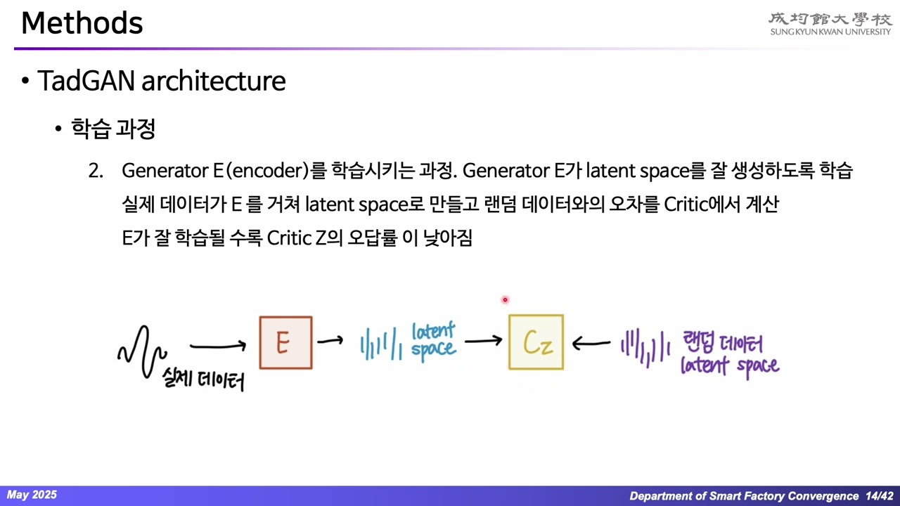

![[Paper Review] TAnoGAN: Time Series Anomaly Detection with Generative Adversarial Networks](https://i.ytimg.com/vi/WkK52d0RWk8/hqdefault.jpg?sqp=-oaymwEmCOADEOgC8quKqQMa8AEB-AH-DoACuAiKAgwIABABGDkgUShyMA8=&rs=AOn4CLDIg5HqAvUyO6_ogb9HAdDuiRTPzA)




This tutorial demonstrates how to implement time series anomaly detection using PyTorch and LSTM Autoencoders. The process involves loading and preprocessing ECG data, defining an LSTM autoencoder model with encoder and decoder components, training the model using the Adam optimizer with L1 loss, and detecting anomalies by comparing reconstruction errors against a threshold. The model learns normal patterns during training and identifies deviations (anomalies) in test data by measuring how well it can reconstruct input sequences.
PyTorch LSTM Autoencoder for Time Series Anomaly Detection
Added:Basic proficiency in PyTorch, including creating custom neural network modules, defining loss functions, and writing training loops.
Fundamental understanding of Recurrent Neural Networks (RNNs) and Long Short-Term Memory (LSTM) networks for sequential data.
Core concepts of Autoencoders, specifically the encoder-decoder architecture and reconstruction-based learning.
Time series preprocessing techniques, such as sequence windowing, scaling, and handling missing values in temporal data.
Dynamic and statistical thresholding techniques for anomaly detection, such as using Extreme Value Theory or rolling statistics rather than static thresholds.
Scaling up to multivariate time series anomaly detection to handle complex correlations between multiple parallel sensor channels.
Advanced sequence architectures like Transformers (e.g., Informer, PatchTST) or GAN-based approaches for sequential anomaly detection.
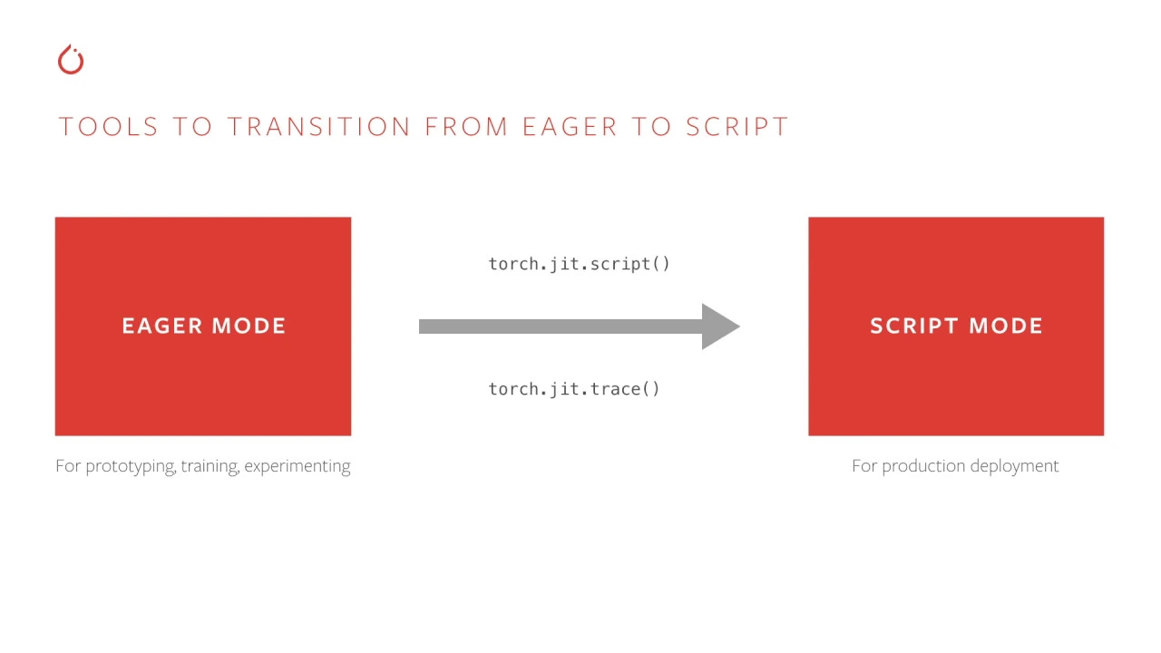
Real-time deployment strategies for streaming inference, utilizing frameworks like TorchScript, ONNX, or integration with data streaming pipelines.
522 views6likes24:19Original Release: 2024-09-03
this command executes the Nvidia system management interface a tool that provides information about Nvidia GPU devices it displays a summary of the GPU status including memory usage GPU utilization temperature and running processes this information is valuable for real-time performance monitoring especially in scenarios involving machine learning models or other GPU intensive tasks it is commonly used in data centers and by developers to optimize GPU resource usage this command uses pip the python package installer to install the af2 panda Library the QQ flag suppresses output messages during installation for a cleaner process the F2 pandas Library converts aif files commonly used in machine learning into Panda's data frames making data manipulation and Analysis in Python easier this command installs or updates The Watermark package in Python using pip the package installer for python the Q flag suppresses output messages unless an error occurs while the U flag instructs pip to upgrade the package to the latest version if it is already installed this command ensures that you have the most recent version of The Watermark tool which is used to display versions of your environment's packages and other relevant information in a notebook or script this command installs or updates the Panda's library in a python environment the exclamation mark indicates it is meant for a Jupiter notebook or a similar interactive environment where shell commands can can be executed the PIP install command is used to install python packages and the options QQ enable quiet mode to reduce installation output while you upgrades pandas to the latest version if it is already installed this command ensures access to the most recent features and Bug fixes of the Panda's Library this code snippet in a Jupiter notebook loads The Watermark extension to provide information about the notebook's environment the command percent reload extension Watermark refreshes the EXT ition to ensure access to the latest features the following command percent Watermark v p numpy pandas torch R2 pandas displays the versions of the specified packages helping to track dependences and ensure compatibility for collaboration and code sharing this code sets up the environment for a data analysis and machine learning project using python it Imports essential libraries for data manipulation visualization and machine learning including pandas numpy sein matte platlet torch and scan it initializes py torch for building neural networks and uses sein and matte plot for creating graphs the directive percent mat plot lib inline ensures that plots display in line in a Jupiter notebook while percent config inline backend. fig format equals Rea improves their visual quality the code configures visual Aesthetics by setting a specific color palette and defining the figure size a random seed is established for numpy and py torch to ensure reproducibility of results which is important in data science workflows effectively preparing the workspace for further analysis or model training this command utilizes G down a command line tool for downloading files from Google Drive the ID flag specifies the file ID which is 16 mco1 V yxl gk4 GK and GM CPU w k kpt when run it fetches the file link to that ID and saves it in the current working directory this method allows users to directly retrieve data files or resources for analysis or development from Google Drive without using the web interface this command extracts the contents of the file named ECG 5000 zip without showing any progress details due to the QQ option which activates quiet mode this allows users to access the files in the zip archive through a terminal or command line interface without cluttering the output with messages making it useful for quickly retrieving files this line of code identifies the suitable device for computations in py torch it checks for the availability of a CA compatible GPU using torch. ca.
isore available if a GPU is present the device is set to ca if not it defaults to CPU this capability enables the program to utilize Hardware acceleration enhancing performance for deep learning model training and inference the code opens two files ECG 5000 tr. and ECG 5000 test.of which are likely data sets in af format for machine learning it uses a context manager to ensure the files are closed after loading their content the function a2p dolo is called on each file converting the a data into a more manageable format likely a panda's data frame consequently the variable train stores the training data set while test contains the testing data set preparing them for further analysis or model training this code combines two data frames train and test in into a single data frame called DF using the append method it then shuffles the rows of DF randomly by sampling all the data in a random order the final step retrieves the dimensions of the resulting data frame showing the number of rows and columns in DF this code retrieves the first five rows of a data frame named DF it provides a quick preview of the data frame structure and contents displaying the column names and data types using head allows you to view a subset of the data set without displaying the entire content which is particularly useful for large data sets this code defines a constant called class uncore normal with a value of one indicating a specific Class Type within a classification system likely for medical or signal processing applications a list named class uncore names contain string representations of various classifications such as normal rnt PVC SP and UB this suggests that the code is designed to categorize or label different data points or events within a larger analysis the constant and the list provide a clear mapping between numerical identifiers and their corresponding descriptive labels this code snippet renames the last column of a data frame called DF to Target it creates a list of the current column names modifies the last name in the list and then updates DF with the new column names this is helpful for specifically labeling a Target variable in machine learning tasks or similar situations this line of code counts the unique values in the Target column of the data frame DF and returns a series with unique values as the index and their corresponding counts as the values this helps assess the distribution of categories in the Target column providing insight into Data balance particularly in classification tasks this code generates a count plot with the sein library to show the distribution of counts for various categories in the Target column of the data frame DF the SNS do count plot function creates the plot and X represents the A's object the extic labels are then adjusted using set uncore extic lables to display the category names from the class uncore names variable replacing default numerical labels for better Clarity this function generates a Time series plot for a specified data set illustrating its average and variation over a defined number of steps it accepts the data a title for the plot a map plot lib access object and an optional parameter indicating the number of steps for the rolling calculation the function Begins by converting the input put data into a panda's data frame it then calculates a rolling mean and standard deviation over the specified steps which Smooths the data and assesses its variance upper and lower bounds are computed based on the rolling metrics resulting in a shaded area that displays the data's variability finally the function plots the rolling main on the designated axis and fills the area between the upper and lower bounds with a light color to highlight the range of variation setting the plot title to the provided class name this code sets up subplots to visualize the average time series data for different classes in a data frame named DF it identifies the unique Target classes and creates a grid of subplots allocating one subplot for each class with a maximum of three columns per Row the code then iterates through each class extracts the relevant data calculates the mean of the features while excluding the target column and converts this mean into a numpy array the function plot uncore timecore series uncore class is called with the main data class name and subplot access to generate the time series plot for each class finally the code removes any empty subplots and adjusts the layout for improved spacing this code filters a data frame called DF to create a new data frame named normal DF which includes only the rows where the target column equals class underscore normal the value of class uncore normal is converted to a string for accurate comparison after filtering the target column is removed from normalcdf leaving only the relevant features finally normalcdf do shape is used to get the dimensions of the new data frame returning a tupal that indicates the number of rows and columns this code filters a data frame named DF to create a new data frame called anomaly DF it selects rows where the value in the Target column does not equal the string representation of class uncore normal after filtering it removes the target column from the resulting data frame finally the shape attribute of anomaly underscore DF provides the dimensions of the new data frame showing the number of rows and columns this code snippet splits the data set named normal DF into training validation and testing subsets it first creates a training set Trainor DF and a validation set Valore DF by allocating 15% of normalcdf for validation while controlling Randomness with a fixed random underscore seat next it further divides the validation set into a new validation set Valore DF and a testing set testore DF where 33% of the original validation data is designated for testing this results in approximately 70% of the data for training 15% for validation and 15% for testing since 33% of the 15% validation set becomes the test set this function takes a data frame as input and transforms it into a list of py torch tensors for machine learning models it first converts the data frame to a npy array array with a data type of 32-bit floats each sequence in the array is then converted into a py torch tensor with an additional Dimension added for compatibility the tensors are set to a floating Point type after creating the tensor data set the function determines the number of sequences the length of each sequence and the number of features by examining the shape of the stack tenses finally the function Returns the data set along with the sequence length and the number of features this process is particular useful for preparing data for models that handle time series or sequential data the code establishes data sets for training validation and testing from different data frames the create uncore data set function is invoked for Trainor DF valcore DF testore DF and anomaly DF it obtains training data sequence length and number of features from the training data frame assigning these to Trainor data set sqor n and ncore features theel validation data set is generated from Valore DF but any additional returned values are ignored similarly testore normal uncore data set is Created from testore DF and testore anomaly uncore data set from anomaly uncore DF with sequence length and features returned from these calls also ignored this structure is commonly used in preparing data sets for machine learning or time series analysis this code defines a neural network encoder using py torches NN module for Pro processing sequential data the encoder comprises two lstm layers designed to encode input sequences into a compact representation the init method initializes the encoder's parameters including sequence length number of features and embedding Dimension and sets up the two lstm layers the first lstm processes the input features and produces a larger hidden State while the second lstm refines this representation to the specified embedding dimension in the forward method the input 10 X is reshaped to fit the expected dimensions for the lstms it passes through the first lstm and the output is fed into the second lstm the last hidden state of the second lstm serves as the encoded representation of the input sequence which is reshaped and returned for further processing or Downstream tasks the decoder class is part of a neural network architecture using py torch extending NN module to process data sequences with lstm layers in the initial Iz ation method it sets parameters such as sequence length input feature dimensionality and the number of output features two lstm layers are created the first maintains the input size and output size while the second lstm has its hidden size increase to double the input Dimension the output layer is a linear layer that converts the output from the second lstm to the desired number of features in the forward method the input tensor is adjusted for lstm processing by repeating it to match the sequence length and reshape shaping it is needed the data passes through both lstm layers and the output from the final lstm is reshaped before being sent to the output layer resulting in the final decoder output this design is well suited for sequential data processing applicable in scenarios like time series prediction and sequence generation the recurrent autoencoder class inherits from NN module in py torch and is designed for creating a recurrent autoencoder model for sequential data processing during initialization it establishes two key components an encoder which compresses the input sequence into a lower dimensional representation and a decoder which reconstructs the original sequence from this embedded representation the dimensions of the sequences features and embedding size are defined as parameters when instantiating the class in the forward method the model processes the input by passing it through the encoder to obtain the encoded representation followed by the decoder to reconstruct the original data the output of the forward me method is the reconstructed sequence facilitating effective learning of patterns in sequential data and enabling the model to generate outputs similar to the inputs this code snippet initializes a recurrent autoencoder model with a specified sequence length number of features and a hidden layer size of 128 the recurrent autoencoder class defines the architecture and behavior of the auto encoder after creating the model instance it is moved to a specified computational device such as a CPU or GPU to enable efficient computation for large data sets or complex models this function trains a deep learning model using a training data set while monitoring its performance on a validation data set over a specified number of epoch it employs the atom Optimizer with a learning rate of 0.001 and utilizes L1 loss for training the model's parameters and loss Criterion are initialized and training and validation losses are stored in a dictionary for analysis the model's weights are saved if the validation lus improves during training during each Epoch the model enters training mode and processes the training data set batch by batch for each batch previous gradients are cleared a forward pass is performed to obtain predictions and the loss is calculated against the True Values gradients are computed and the optimizer updates the model weights accordingly collecting training batch losses after training the model switches to evaluation mode processing the validation data set without updating weights to cons of memory average training and validation losses are computed and recorded if the validation loss is the lowest encountered the model's weights are updated to reflect this Improvement at the end of the training process the model reverts to the best weights found and returns alongside the recorded history of losses for performance evaluation this code calls the function train underscore model to train a machine learning model the function requires several parameters including the model to be trained a training data set a valid validation data set and the number of training iterations which is set to 150 it Returns the train model and its history which typically includes metrics such as loss and accuracy over the training Epoch for post-training analysis this code uses Matt plotti a plotting library in Python to visualize the training and validation loss of a model across multiple Epoch it creates a new figure and retrieves the current axis the code plots the training loss from history train and the validation loss from history vow the y-axis is labeled loss and the x-axis is labeled Epoch a legend is included to distinguish between the training and validation loss lines and the plot is titled loss over training EPO finally it displays the plot this code effectively visualizes changes in the model's lustering training aiding performance analysis this code saves a py torch model to a file called model. pth using the torch. sa function it takes the model object and the design file path as arguments after executing this line the model's current state will be stored on disk enabling you to load and use it later without retraining this snippet outlines the process of downloading a file and preparing a machine learning model it begins by using GD down to retrieve a model file named model. pth from Google Drive specified by its file ID next the model file is loaded into a py torch model object finally the model is transferred to a specified device typically a CPU or GPU to prepare it for inference or training this setup is standard when working with pre-trained models in py torch the predict function generates predictions from a machine learning model using a specified data set while calculating the associated losses it begins by initializing lists for predictions and losses and employs L1 loss as the loss Criterion which measures absolute differences between predicted and actual values the loss is summed across all data points move to the appropriate device such as a GPU or CPU within a no- gradient context the function sets the model to evaluation mode to adjust certain layers like Dropout and batch normalization for each sequence in the data set it transfers the true sequence to the designated device and generates predictions by passing this true sequence through the model the loss is computed by comparing predictions with True Values using L1 loss and the predicted values are flattened and converted to a numpy array before being added to the predictions list the loss value is converted to a python float and added to the losses list the function then Returns the predictions and losses as separate lists which AIDS in analyzing the model's performance on the data set the code calls a predict function with a machine learning model and a training data set which returns two values the first value is ignored while the second value losses contains the loss metrics from the model's predictions on the training data the code then uses the sein library to create a distribution plot of the losses data configuring it to have 50 bins and including a kernel density estimate Line This visualization AIDS in understanding the distribution of model losses and identifying patterns or anomalies this line of code defines a constant named threshold with a value of 26 constants are used to represent fixed values that remain unchanged throughout the program the uppercase naming convention indicates that this value functions as a global constant which may be U ized later in the code for comparisons controlling flow or setting limits depending on the context this code Begins by calling the predict function with a model and a test normal data set which produces two outputs predictions representing the model's predicted values and pred unders scol losses containing the errors associated with those predictions it then utilizes cin to create a distribution plot of the pr underscores the parameter been set to 50 divides the data into 50 intervals for the histogram while KD set to True overlay is a kernel density estimate line on the histogram this visualization AIDS in understanding the distribution of prediction losses thereby facilitating the assessment of the model's performance regarding prediction error this code counts the number of predictions in the prore luses list that are less than or equal to a specified threshold it uses the sum function with a generator expression that iterates over each prediction loss in PR underscore losses evaluating if each loss meets the threshold condition the sum of these evaluations is stored in the variable correct following this the code prints a message showing how many predictions are classified as correct normal predictions along with the total number of items in the testore normal uncore data set this provides a clear insight into the model's performance in correctly identifying normal cases based on the defined threshold this line of code creates a new data set named anomaly uncore data set by slicing testore anomaly uncore data set to match the length of testore normal uncore data set this ensures that anomal uncore data set contains the same number of samples as testore normal underscore data set which is useful for balance testing or analysis particularly in machine learning where class distribution matters this code snippet performs two main tasks it first calls the predict function with a train model and an anomaly data set which computes predictions and their corresponding losses the predictions variable stores the model's output while prore losses holds the loss values that indicate the accuracy of these predictions the second part utilizes the sein library to visualize the distribution of prediction losses the SNS doist plug function creates a histogram with 50 bins for the pr underscore losses and overlays a kernel density estimate to illustrate the probability density function of the losses this visualization AIDS in understanding the distribution of prediction errors providing insights into the model's performance on the data set this code calculates the number of correct anomaly predictions based on a threshold it iterates through a list called prore losses which contains prediction loss values and counts how many of those values exceed a specified threshold the result is stored in the variable correct and it finally outputs a message showing the number of correct predictions along with the total number of entries in anomaly underscore data set providing a clear indication of prediction accuracy for anomalies the plot underscore prediction function takes four parameters data a train model a title for the plot and an X object for drawing it starts by calling a predict function that generates predictions and calculates the loss using the model and input data the function then plots the true data on the a object and labels it as true it also plots the reconstructed predictions labeling this line as reconstructed the plot title is set to include the specified title along with the formatted L value finally a legend is displayed to differentiate between the true data and the reconstructed data this code creates a 2x6 grid of subplots using matte plot liet a widely used python plotting Library the Fig siiz parameter specifies the overall dimensions of the figure as 22 in wide and 8 in tall the first Loop processes the first six entries from the testore normal uncore data set using the plot uncore prediction function to generate predictions from the model and display them in the top row of the grid with the title normal the axis a zero I indicates the sub plots position in the first row the second Loop performs a similar function for the first six entries from the testore anomaly uncore data set plotting them in the second row under the title anomaly finally figure typeor layat is used to optimize subplot parameters for a cleaner layout ensuring that titles and axes do not overlap
Up Next

11:08
Metrics for Anomaly Detection: Precision, Recall, Rank Power
@JosephRivera517
196 views•2021-08-08

57:48
Secure Multiparty Computation (MPC): Foundations & Challenges
@SimonsInstitute
7.3K views•2015-05-28

13:03
Bypassing Tor Censorship: Bridges and Pluggable Transport Guide
@Coding_ForEveryone
397 views•2024-06-11

18:41
Neural Networks Explained: Math, Layers, and Learning Fundamentals
@3blue1brown
21.9M views•2017-10-05
Related Study Plans & Knowledge Roadmaps
Structured learning paths in Artificial Intelligence
artificial-intelligence
Aligning LLMs: DPO, TRL & Custom Datasets
01Foundations of Python & Machine Learning
02Transformers and Large Language Models (LLMs)
03Aligning LLMs: SFT and RLHF
+ 3 more learning modules
24h6 modules
Explore Roadmap
artificial-intelligence
Federated Learning: PyTorch, Flower & Privacy
01Python & Machine Learning Foundations
02Deep Learning Basics with PyTorch
03Introduction to Federated Learning
+ 2 more learning modules
35h5 modules
Explore Roadmap
artificial-intelligence
Securing LLMs: Guardrails AI & NeMo Gateway
01Introduction to LLMs, Python, and APIs
02Understanding LLM Vulnerabilities & Threats
03Defending LLMs with Guardrails AI
+ 2 more learning modules
15h5 modules
Explore Roadmap
artificial-intelligence
Building Recommenders: Two-Tower & Vector DBs
01Foundations of Python & Machine Learning Basics
02Introduction to Recommender Systems
03Deep Learning & Representation Learning
+ 3 more learning modules
75h6 modules
Explore Roadmap