
![[UFMS Digital] Redes Neurais - Módulo 1 - Unidade 1](https://i.ytimg.com/vi_webp/PQsvqlre7hE/maxresdefault.webp)



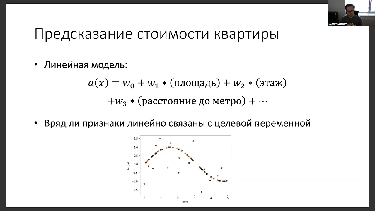


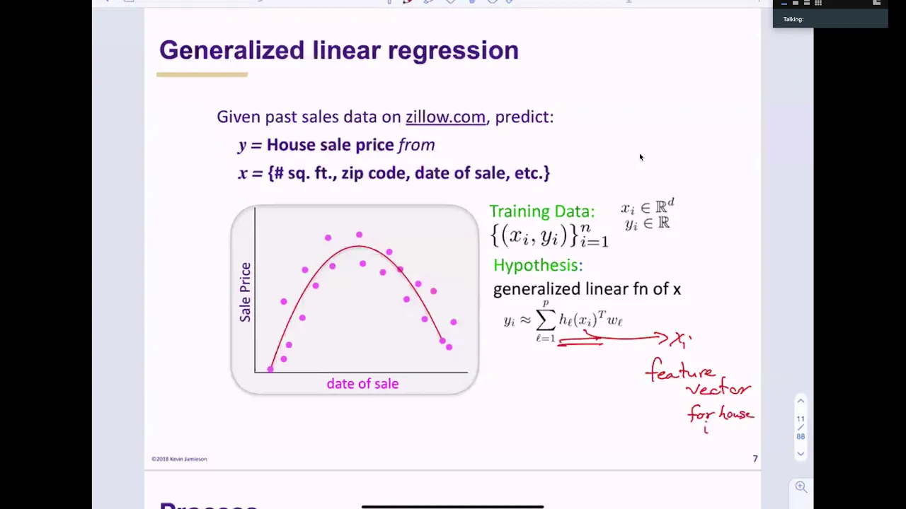



![แนวคิดเชิงเส้นในตัวแบบเชิงเส้นนัยทั่วไป [Ep6.]: เติมเต็มชีวสถิติ...อย่างมืออาชีพ](https://i.ytimg.com/vi/RsXAaEgAC-o/maxresdefault.jpg)


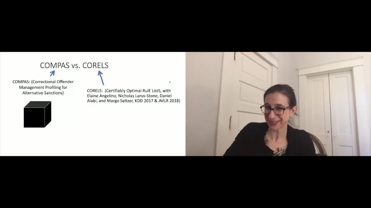



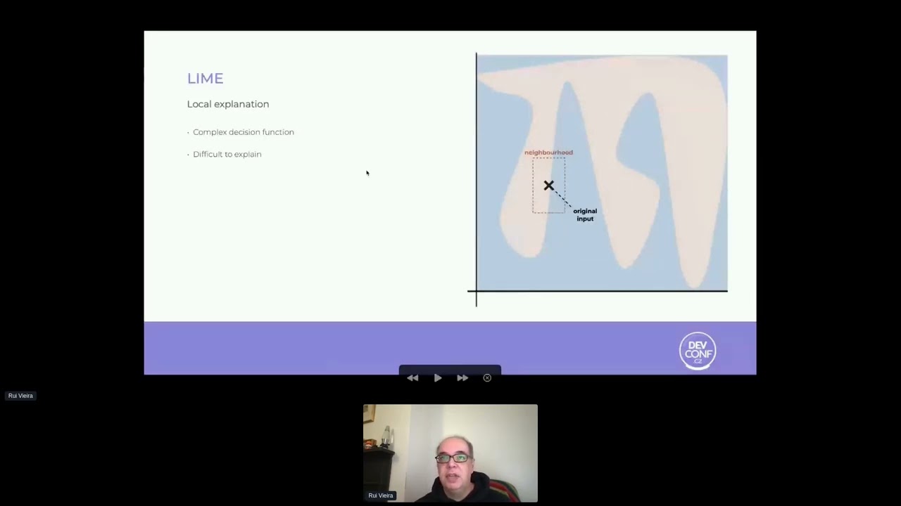


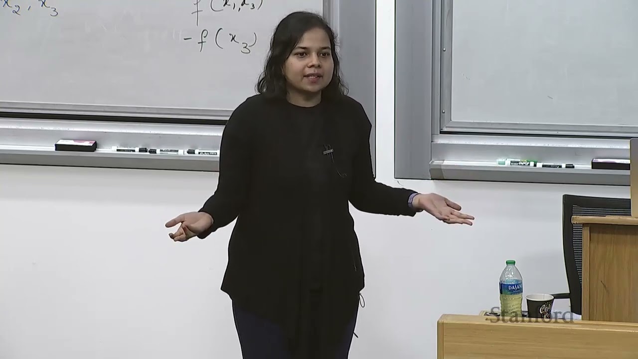







Inherently interpretable machine learning models are designed to be understandable by construction, rather than requiring post-hoc explanation. Key approaches include: (1) Rule-based models like Bayesian Rule Lists (2016) that generate if-else-if rule lists using generative Bayesian processes with Metropolis-Hastings optimization, and Interpretable Decision Sets that optimize for sparsity, distinctness, precision, recall, and class coverage; (2) Risk scores that assign point values to conditions and sum them to predict risk levels, formulated as mixed integer programs; (3) Generalized Additive Models (GAMs) that model outcomes as additive combinations of shape functions for each input variable, with GAM² extending to pairwise interactions; (4) Prototype-based models that identify representative instances from data to classify new points; and (5) Attention layers in deep learning that highlight which input features influence each output decision, providing interpretability through explicit attention weights.
Machine Learning Explainability: Inherently Interpretable Models (Stanford Seminar)
Added:so in terms of inherently interpretable models we started our discussion about you know things like shallow trees or like simple linear models or simple rule-based models and so on uh in this module for the next 40 minutes or so we'll do a quick overview of some of these approaches so let me start by saying that I am not going to touch on the very basic sort of linear models or regularized linear models with like L1 or l0 or L2 style regressions regularized regressions but instead I'm going to start from something like around the year 2014 2015 uh since when since then there has been more renewed interest in you know sort of like building inherently interpretable models exploring newer ways than what we had with respect to you know previous work in 70s and 80s right so what I'm not covering is few things so just linear models linear logistic regression regularizations on top of them and then decision reconstruction using greedy approaches so those are the things that I'm going to sort of put a pin on and assume some familiarity for all of you but I'll start from the year 2015 and go over some of the approaches that came since then okay does that sound good all right okay so uh again as I was saying so with the renewed interest recently a lot of approaches again the constructs is probably what I would encourage all of you to take away from some of these discussions so the people have tried to build several kinds of inherently interpretable models so one is rule-based models the other is risk scores and I'll explain what they are in a little bit and then there is generalized relative models which had gained a lot of popularity recently and then there are prototype based models okay so let's go over each of these oh and also attention-based models all right Okay so let's go to the first set of approaches that is the rule-based approaches uh and you know I'm going to first talk about a couple of approaches in this categories before I move on to another one uh this approach called Bayesian ruleless was introduced in 2016 uh by Ben Latham and Cynthia Rudin and this was basically an approach that is I mean the output of this approach looks something like this right so it's a sequence of if else if rules and this is actually the output that they get with their method uh as a classifier for stroke prediction right so this is basically like they were working with some doctors and Healthcare experts to design models that can be used to predict Strokes in advance or stroke risk in at once and the requirement in those settings is that doctors want to precisely see the rules that can be used to sort of employ as they go you know in their day-to-day decision making right so they didn't want any kind of complex models they wanted something as simple as this but also they wanted something accurate right so this approach is kind of motivated by that scenario uh so what exactly is their approach right so their approach is basically proposing a generative model uh which is designed to produce these kinds of if else if lists and the way they Design This generative model is by striking a balance between accuracy interpretability and computation and I'll go into some more details about this approach but you know you could look at or anyone could look at that particular offensive list that we saw and say wait why are they just not using other similar models for example what about decision trees like cards c5.0 C 4.5 why are they not using these kinds of models right the reason or at least what the paper argues is that these kinds of models employ greedy based approaches so while greedy methods as we all know are efficient they can often get stuck in local Minima right so the argument that this paper makes is that it is is computationally great but you know the resulting solution is not going to be perfect in terms of accuracy or interpretability so that's why they sort of like put forth that there is a need for new methods to even generate things like rulers from scratch okay so for those of you who are familiar with Bayesian models here is what their generative model or their generative process looks like if you think about it and for those of you who are not familiar there's no need to worry too much all that goes on in generative models or these kinds of Bayesian topic modeling style approaches is that you sort of assume a particular process that generates the data and then you have a bunch of unknown parameters as you assume this process and then you work backwards and then try to estimate or learn those unknown parameters using different techniques right so that's the basic you know Intuition or concept behind generative models so what is this particular generative model trying to do so essentially the generation process says you know first of all pick a list length so how many rules are there in the list you know we sample that number and then we basically sample a default rule which will apply for 3 things that no other rule is going to apply for and then we are going to sample the M different other rules in our offensive set of the list and for each rule what we do we basically sample the cardinality of the antecedent which is the left hand side of the rule how many predicates are in the left hand side of the rule and then we basically sample the predicates on the left hand side of the rule right so you sample the number and then you sample the predicates and then of course you sample what should be on the right hand side of the rule right and then for then the observations will be generated from these sampled rules as you know find find the rule that actually applies to this instance in the data and then if no antecedents apply or no rules apply then you basically give it the default rule otherwise you sort of sample a class label based on that rule that applies to this instance right so that's the high level if we were to sort of think about constructing these rules that's intuitively how you would think about this kind of a process okay so I want to note few things here so one is the the sort of sampling the predicates or the conditions and when I use the word predicate I basically just mean you know these conditions are the predicates right so it's like if transient is basic or if transient uh ismic attack that's the condition or that's the predicate all right so a here is the set of pre-mind antecedents so what do I mean by that is whenever they are trying to sort of pick the left hand side of the rules they're actually selecting from a set of candidate left hand sides that are already available okay so they use some sort of like frequent items at mining for those of you who are familiar with a prairie style algorithms so they kind of use that to sort of determine what are some of the frequently occurring patterns in the data and then try to pick left hand sides from those okay so there is a candidate set and they try to pick from it so now just at a very high level for this kind of a generative process we use something called as Metropolis Hastings algorithm it's essentially like for those of you who are familiar with mcmc or Gib sampling method so this is essentially one of those classes of algorithms and using this they go back and estimate all the parameters in that generative process that they don't know right so for example before constructing the list you don't know what will be the cardinality of the antecedent or the number of predicates of antecedent of some rules or you don't know how many rules you're picking right so but using this process they go back and you know sort of learn those and then build the list yes that's the high level idea all right so one of the major uh sources of practical feasibility here is the set of pre-minded antecedents or pre-bind left-hand sides of these rules and that basically helps them reduce the model space because you are essentially searching over those rules only in order to find your final list right so if your candidate rule set is small then you basically have smaller search space to look at right so they can control the complexity of the problem through that right and as long as this set of pre-minded antecedent list is expressive you will be able to find an accurate enough decision list uh plus you know having that said to be small can also help with like better generalization as well right so you need to choose that set carefully in order to find a good or an accurate decision list with this method okay any thoughts questions all right okay so the next approach which kind of tries to simplify this process a bit more further and also makes it more efficient uh and also adds some tweaks on interpretability which I'll also discuss a bit more in our analysis section is interpretable decision sets and you know this is like an example decision set classifier for disease diagnosis task on a particular data set right so what immediately kind of strikes to you is instead of if else if rules there is a set of unordered if then rules here so that's the main difference in terms of how the rules look like you would be surprised to know that even just a change in the construct from if else if to if then already changes significantly how people perform certain tasks for example and I'm going to talk about this lot more in our analysis section to show how even simple changes in how an interpretation looks right can have big differences in terms of like you know let's say if a doctor is looking at these rules and trying to make some decisions and so on the cognitive load that is incurred with small changes can actually be pretty big right so while computationally we might be like oh that's a list you know there is ordering there's a set there's no ordering like that's the difference but like these things have a lot of impact and we'll talk about that a bit more later so this approach will also hopefully make it clear to you as to what exactly is the deciderator Behind these kinds of rule approaches that are being used uh to construct these rule-based models again in a renewed fashion since 2015.
um so this is what is the set of criteria that this approach is focusing on uh which is you want to account for recall Precision distinctness of the rules sparsity in the rules and then covering all the classes right and recall and precision is important for accurate predictions and distinctness parsimony and covering all the classes is important for interpretability right so just to go over some of the terms here and just bear with me as we do this because these are the building blocks of a lot of the things that we'll talk about later so then we are going to just skim through these details and say oh we refer to them then okay all right so the objective function in this case as we were saying it's trying to sort of Encompass five different criteria right so uh parsimony or the sparsity is basically trying to ensure that there are fewer rules in the rules set so now our goal is we have to pick from a candidate set of rules that we have we need to pick a subset of some K if then if then rules and then that will become our classifier right and the first Criterion in that is we favor fewer rules so we want to either sorry minimize the number of rules which is denoted by size of r r maximize the negative of that so that's essentially what you see is that expression there okay and also fewer predicates which is basically the number of conditions in the rules that should also be smaller so we want to minimize that or maximize its sort of complement or it's negative right now in terms of distinctness because what we are looking at here is trying to find a set of if then rules we want to ensure that the points being covered by these set of rules is minimal right or covered by multiple rules in this set of rules is minimal because otherwise you are essentially just creating duplicate rules which you don't need right so you are trying to basically minimize two Notions of overlap which is intra class overlap and Inter class overlap so basically the point is that the number of points that satisfy more than one unrul should be minimized okay so that's what this expression is trying to capture and then the next one is class coverage which is you are basically checking to see that there is at least some rule corresponding to a given class or any given Class C so that Minority classes for example in the kinds of data sets we are looking at like the healthcare data sets some rare cancers they are like present in such tiny number of samples in the data that classifiers might often just ignore them because it doesn't matter to their overall accuracy right but here we are sort of forcing that to happen and we want every class to be represented in some Rule and then of course there is the Precision piece where you're trying to minimize incorrect covers right so basically we want to minimize for each rule that we pick in this set of rules the number of points which satisfy the rule but do not belong to the class that the rule is assigning the point to right so that ensures Precision which is in important for accuracy and then recall and the way we are sort of trying to enforce recall is that you encourage each point to be covered by at least one rule in the set that you produce right so for example that correct cover that you see there that's basically capturing the number of data points which satisfy uh s and also which is the rule is and also belong to the class C right so you're basically trying to ensure that no point is left out from this covering process okay all right so putting it all together what you see is you can basically combine these put it into an optimization problem you know essentially you'll get some kind of Arc Max problem like this and then a summation over all these factors so the property of this kind of an objective or the set of properties of this kind of an objective is that this turns out to be something that's called a non-normal non-monitode and submodular optimization problem okay so without going into too much details because you know that's not the point of this conversation uh maximizing such a problem turns out to be NP hard but the good news is there are some approaches which can provide reasonable approximations and we can use those to efficiently solve this objective right in fact faster than what the Bayesian rule list was trying to do okay all right so with that I think we are kind of pretty much covered like some of the uh key approaches that were proposed as the interests in rulers and rules that's got rejuvenated somewhere around 2015.
um there are also several other classes of inter interpretable models so next one is called as risk scores uh so risk scores are basically things that look like this so I'm going to just let you guys see this as a pause for a minute okay so what you see here in these kinds of risk score lists is that for each condition you are assigning points for example if the number of Prior errors is greater than or equal to two that's worth one point right and you know if your age it release is greater than or equal to 40 that's actually a negative one point so you're trying to sort of create this kind of scores associated with conditions and at the end of the day you will just sum up all those scores and the resulting score will tell you how risky it is for example for a defendant to be released or how much of a risk there is in a person defaulting on a loan and things like that right so it's almost like saying if this condition holds add a point and you know as these conditions hold key padding points what is the total and the total will tell you how risky the person is okay so this kind of a construct is actually pretty popular both in medicine and criminal justice like uh I myself collaborate with doctors and folks in criminal justice and they are very comfortable with this kind of risk course because all they have to do is just kind of go through that checklist and assign points and then they get a risk right risk score so that's why they're pretty popular in fact the existing models of risk scores that are out there quite a bit in practice in domains like medicine and criminal justice are like handwritten or hand-drawn risk or checklist which have been sort of made up by domain experts or doctors or you know lawyers and judges of course they're using their domain expertise in coming up with those lists but essentially they sort of prefer these kinds of checklists with scores uh quite a bit so there's something that naturally comes to them in terms of utility Okay so how do we now construct these kinds of risk score checklists using data right so that's the problem or that's the question that was dealt with by Austin and Rudin in the year 2016. okay so this is roughly the kind of problem that they formulate it turns out to be a pretty complicated problem to actually solve correctly accurately so we'll get to that a bit later but essentially if you see what this is trying to do is that so you're trying to basically uh formulate or come up with this kind of set of conditions and corresponding scores such that you are basically minimizing two terms so the first one is basically ensuring that your scores work out so the scores that you are applying and then you will sort of use those scores to then convert them into the probability of risk associated with someone let's say right so the scoring mechanism the first term will ensure that that score scoring mechanism or the scores you are assigning to each of the you know the predicates in your risk score list uh actually map to the uh precise risk in practice are the real estimates of the risk in the data so that's that's what that last term is doing in the objective and then the second term you are essentially trying to sort of minimize the number of the predicates or the terms that will get on to this risk score checklist right so you don't want the checklist to be you know having like 100 attributes there right so you want to minimize that so that's what that second term which is a regularization term is doing and then of course there could be a bunch of other constraints on how you will pick these uh conditions that you see in the risk score checklist and also the scores that you assign to them for example there might be a condition that don't assign continuous valued scores the scores that you assign should be integers because those are more interpretable right so you can think of them as 1.2 point but not as 1.73 or something right so uh there could be a bunch of such constraints both on what features you're picking and also what scores you are assigning to them that is encoded by the condition there right so the above when we put together some of the more sort of practical conditions into this problem setup uh turns out to be a mixed integer program and it is optimized in this particular work using a cutting plane method and a branch and mount technique so it does not have an easy solution but I think we'll leave it at that okay all right so the next class of models is the generalized additive models um and okay so this is the class of models which basically produces outputs like this so what you are essentially seeing is that you kind of see what are called as shape functions associated with input variables so what this is showing is demand is your outcome variable okay and each of the variables you see on the x-axis are your input features so this is kind of showing how the outcome variable will change as a function of each of the input variables right so as R increases what happens to demand and as you know temperature increases what happens to demand and so on and by the way these are not just plots from the data this is actually the output of the method that is generalized relative models okay so it shows you how the output can be modeled as different functions of input variables so the output in this case is essentially a summation of all the curves that you're seeing here okay it's like an additive combination so just to show you a precise mathematical form of this uh so for example the first row here is essentially like a linear regression model right so your Y is basically this kind of a additive or like a linear combination of different features that you have and then we go one step up to a generalized linear model uh where you can take a function of Y and then model it as a linear combination of different input features right then we can think of an editor model where your y will just be an additive combination but of different input of different functions of the input variable right so each input variable you can learn a separate function over it and then the additive combination of that will give you y now a generalized version of that is basically a generalized additive model where you can take a function of the output variable that is g of Y and then think of that or consider that to be this kind of an additive combination of you know input functions functions of in different input variables okay and of course if you want to make the model more complex you know your Y is basically just a function of all the input variables and that could be an arbitrarily complex function right so think of deep neural Nets and so on which fall into the last category so the stable also kind of tries to summarize some of the knowledge that we have been thinking about so if you think of a linear model it's just a bunch of coefficients associated with each feature we multiply the feature where the coefficient add everything up we get the output right so the interpretability or the intelligibility factor is high accuracy may not always be high of course depending on the data it might but it may not be as high now if you think of the generalized linear model which is something like a logistic regression in that case also your intelligibility or ability to see five weights and then see what they're doing that is good but again accuracy may not always be good right and then the third row is the additive model where you are just thinking of additive combination of different functions your intelligibility is probably a bit worse off than just seeing you know the actual variable itself because now we are seeing a function function your accuracy might improve a bit though right and the same is the case with generalized relative model so you are seeing complex functions now so your interpretability is probably not as high as just thinking of it as one variable and its weight but at the same time it helps with accuracy a bit right okay so uh Gams and Gams squares I guess that's how they're called so these have again become popular starting 2015 2016.
so Gams are essentially what we just saw so they sort of model these first order terms and their like additive combinations of the functions of the different input variables gam square is basically going one step further and it is also considering pairwise interactions between features right so the claim is that these kinds of shape functions that you saw earlier that are produced by these approaches are interpretable and we'll talk about that as well in just a bit right so how to learn these kinds of models so the idea here is that given that you're trying to fit a function on each input variable and then do an additive combination of it so you basically represent each feature or each component as a spline and then you basically use a least squares formulas and then run an optimization procedure to sort of balance smoothness of the spline as well as the empirical error right so that's that's how you go about it and then with gam Square you also have the higher order interaction terms to consider so in this case you first build a gam which is without the interaction term take the residual error okay and then rank all possible pairs of interactions uh in the reset dual and basically try to pick some top K interaction pairs that are contributing to the residual using some sort of feature selection type approaches and then uh like even cross validation right and then just pick those top K Pairs and now try to again repeat this learning procedure where you're basically representing each the pairwise interaction term as a spline and you're just sort of using a least squares formulation to fit it okay so yeah if some of this feels a bit for fuzzy that's fine these are details of how exactly people are trying to learn such models but the important piece is the construct that you saw which basically looks something like this and you know the claim is these kinds of things are actually interpretable um I think I'll just uh sort of do a poll here to see how many of you think this is interpretable show off hands okay that is some of you all right uh what about the rest how many of you think it's not interpretable let me see if there are people who are undecided oh there are some undecided folks okay uh so why do you think it's not interpretable I think maybe there are one or two features right and what do you feel about thinking about this as the whole outcome variable is some kind of additive combination of all these shapes right so I think I understand the sensitivities of each variable but not the combined effect of materials across multiplication right so I think the the sort of intelligibility or the interpretability I know we are using these terms and what Loosely but of Gams has been debated quite a bit uh so again there are pieces of it that make it interpretable which is you can kind of see how the output would vary as a function of individual input variables right but at the same time thinking about all the variables in one shot or in conjunction and then thinking what their effect would be on the output is a little hard to Fathom from something like this right so there have been debates about like whether this should be considered interpretable or not in fact I think you know there is a death of like doing more user studies to actually check if some of this is considered interpretable if so by what kinds of users and so on okay all right so with that I'm going to keep us moving and let's talk a little bit about prototype based models okay so first from here on we are actually also jumping into some more complex aspects but I'm first going to describe a very simple approach for what would be a prototype based models and then we'll see how to sort of make deep learning models interpretable by incorporating you know prototypes or some other constructs okay all right okay so the goal with this particular like the basic problem we are considering here is to identify K prototypes or instances from a given data set such that if there is a new instance we can use these prototypes to assign labels for that instance right so you want to pick some representative points in the data set such that if you give me a new data point I should be able to compute the nearest neighbors among these representative points and assign the label of that nearest neighbor and that should be the correct label for that new data point so in some sense I'm trying to build a classifier through these representative data points okay is that clear right so the way to sort of the way at least this paper goes about this problem is that you consider each instance to cover some Epsilon neighborhood around it right like an Epsilon ball around it we consider that each instance sort of covers that neighborhood okay which means and cover means if a point lies within that Epsilon distance from the uh From Any Given instance then you say this point belongs to the Epsilon neighborhood of that instance and I'll show you pictorially in just a little bit right so once you associate this kind of a neighborhood with each instance now what you have done is you can sort of see the analogy between this and a rule right so earlier we were trying to come up with a subset of rules in the rule set that we discussed about or the interpretable decision sets that we discussed about we were coming up with a subset of rules that can cover all the points in the data and also be accurate classifiers right so similarly we are just replacing the construct of the rule now with a prototype or an instance and an instance is set to cover all the points within the Epsilon ball neighborhood around that instance right so for example and then once we see this sort of deduction or reduction to this problem we thought about earlier as soon as you define this neighborhood you can apply all the optimization problem that we talked about earlier in the context of rule sets and then find a subset of prototypes that maximally cover the data but is also accurately assigning labels to the points that are getting covered right so just to show some pictorial representation of this and the value of this Epsilon that defines the neighborhood can be given by an end user right so this is basically showing for different values of Epsilon if if we pick certain prototypes what are the neighborhoods that they're covering right so if Epsilon is small you will end up picking a lot of prototypes because you know it's only covering a small portion of the data each prototype is only covering a small portion of the data but as you increase the value of Epsilon you will end up picking fewer prototypes because each prototype covers a larger chunk of the data right and then so essentially what you have built is some kind of a nearest neighbor classifier and you have sort of took some prototypes out for building such a classifier all right so this is another popular class and this kind of nicely feeds into a discussion on so so far we have been talking about you know we want simpler models simpler constructs how do I learn rule lists and Rule sets and you know Gams and you know simple prototype based models so I'm sure some of you are wondering okay when will we get a deep learning right so the all these seem like nice and simple models but these are not going to help with my accuracy I want to run deep learning models so what about interpretability there right so here we are jumping into that territory foreign okay so this is basically and there are few approaches which try to do something like this the idea here is that you can make deep learning architectures interpretable by essentially introducing these kinds of layers right so there's a prototype layer followed by a fully connected layer so you can augment these two layers almost towards the end of a given neural network architecture and try to get some interpretability uh in terms of the predictions being made okay so this particular the specific architecture that you're seeing what it has is this first part is basically what is like a auto encoder right and then you take the output of the encoder and then you pass it to the Prototype layer and the fully connected layer and then you get the output and we'll go into the details of what each layer is doing okay so uh yeah so like let's say our input has a dimensionality of you know P right so it's all real numbers so there's the vector uh of real numbers and of Dimension B and then that passes through the encoder and then it gets transformed into you know RQ which is basically a q dimensional Vector of real numbers and you know Q is typically less than P right so for those of you who are wondering what exactly this component is think of it as essentially it's creating a low dimensional representation of your input right so in some sense you are trying to reduce the dimensions in your data while preserving the most important information okay so you're doing that in the first component and then you are inputting a q dimensional Vector of real numbers to the Prototype layer and what is the Prototype layer doing the Prototype layer is actually responsible for computing or learning the Prototype types and more specifically each node in the Prototype layer is Computing this value right so for example P1 is Computing so given an input data point x we got this Z which is the transformed version of X and then each of those nodes in the Prototype layer is Computing the sort of this L2 Norm difference or you know you can think of it as the distance between Z and P1 okay so between the transformed input point and the Prototype that it's learning or it is currently learned right so in some sense each layer is just outputting the distance between the input point or some transformation of it and then the Prototype chosen so far okay all right so now that that's the case the dimensionality of that Vector will be M so that is basically you get one distance value with respect to each prototype right so you get you know first node is Computing the distance between Z and P1 second node is Computing the distance between Z and P2 and so on you get one scalar value from each of those nodes so the entire output of that layer will be M different values okay all right so then the fully connected layer is essentially Computing awaited some of these distances right so you got the distances now you can make these distances the combin the weighted combination of these distances using the uh this fully connected layer here and then of course so that will sort of take the dimensionality from RM and you're sort of multiplying that before with w and so basically that will end up being a k dimensional vector and that in turn can be passed on to the soft Max layer in order to Output probabilities over K classes right so basically what you're doing in sort of all these details is that you're essentially trying to so normally deep neural networks would basically have let's say this component none of these two layers and then you go straight there right but you're introducing a couple of interpretability layers there are mainly the Prototype layer there so that for every instance you also have a prototype that sort of says something like oh I made this prediction on this instance because it looks like this prototype does that make sense so that's the thing that we are trying to get to uh here by adding these kinds of layers okay right Okay so I think we have a little bit more time before the break and I'm going to cover this as well so the last is attention-based models again this has gained a lot of popularity in recent times so the idea is just like we were thinking about adding these prototype layers uh to deep neural network architectures here we are thinking of adding another kind of layer which is called as attention layer right okay so just to illustrate this let me first show you this example of a machine translation task okay so there is nothing uh interpretable here we have not yet introduced anything but this is an example of an architecture of a models that people use to do machine translation okay so the idea here is that so there is your input you are trying to translate this sentence from English to French okay so there are three tokens in your input and each token is passed through an encoder which will basically generate some kind of a hidden state representation for that token okay so that's what this side is doing all right and as you can see the hidden state representation for the second token depends on that as well as you know this input right so both are the inputs here so in some sense you are trying to basically take each word and then get some Vector representation of that word through some process like just think of it in that abstract way okay so now once this encoder is sort of built uh the next part is that there is a decoder on the other side which is basically so there is a context Vector in between I think for the purpose of this architecture you could assume that c is basically just uh taking the value of H3 which is the encoded representation of the last word there okay so I think there are architectures which do use that and some functions of H3 and so on but let's just assume C is H3 okay and C is often referred to as the context Vector because it is trying to capture some context about the input okay all right so now the next set of layers that you have is the decoder and that takes c as input and then tries to generate a hidden state representation for each of the output words and then you know once you generate that hidden straight presentation for say the first word in the output then conditioned on that hidden state representation you can generate the actual word right so that's how machine translation happens with models like these okay so now uh attention layers how to add it in this kind of an architecture right so before I describe exactly what is attention here the change that you hopefully notice from the previous slide to this one is that we kind of added some complexity to the context Vector right so what we are doing is now the encoder has remained the same the decoder has remained the same the context Vector is no longer just C so we now have like separate context vectors corresponding to each token of the output right so the way we introduce interpretability into this is as follows so the context Vector corresponding to each hidden representation of an output token uh which is Si is basically the hidden representation of the output token I so the context Vector will be modeled as this kind of a combination which is a i j and then h j right so in some sense what you are doing is you're representing each context Vector as some kind of a combination of each of the Hidden representations from the encoder side so you're no longer saying I am just going to take H3 and then all the decoder pieces will depend on just H3 what you're saying is my context will be some combination of these three and I will learn what that combination is and that combination will tell me the importance of each of the input words in generating each of the output words right so that's exactly what you're doing when you basically add this kind of a term there okay so in some sense the AIG that we have introduced there it captures the attention placed on input token J when determining the decoder hidden State SI right so in some sense how much does the output word I depend on each of the input words J that's what is captured by a i j right and that is basically the notion of attention weights and that basically describes the importance of each of the input features in these kinds of Networks
Up Next
Shapley Values in Machine Learning: Feature Attribution
@adataodyssey
30.5K views•2023-04-03

Secure Multiparty Computation (MPC): Foundations & Challenges
@SimonsInstitute
7.3K views•2015-05-28

Stanford CS229: Building Large Language Models (LLMs) | ML Lecture
@stanfordonline
1.8M views•2024-08-27

Neural Networks Explained: Math, Layers, and Learning Fundamentals
@3blue1brown
21.9M views•2017-10-05
Related Study Plans & Knowledge Roadmaps
Structured learning paths in Artificial Intelligence